Example data sets

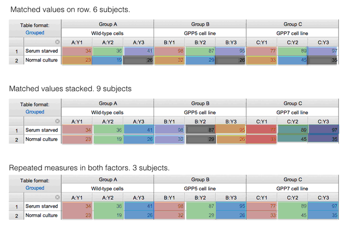
To create the examples below, I entered data with two rows, three columns, and three side-by-side replicates per cell. There were no missing values, so 18 values were entered in all.  

I analyzed the data four ways: assuming no repeated measures, assuming repeated measures with matched values stacked, assuming repeated measures with matched values spread across a row, and with repeated measures in both directions. The tables below are color coded to explain these designs. Each color within a table represents one subject. The colors are repeated between tables, but this means nothing.

ANOVA tables

The table below shows the ANOVA tables for the four analyses. The values below are all reported by Prism. I rearranged and renamed a bit so the four can be shown on one table.

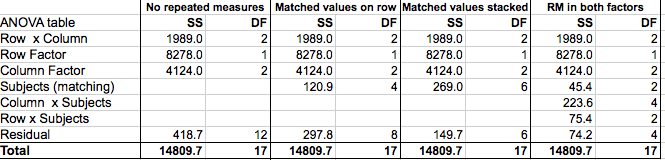
Focus first on the sum-of-squares (SS) column with no repeated measures:

•The first row shows the interaction of rows and columns. It quantifies how much variation is due to the fact that the differences between rows are not the  same for all columns. Equivalently, it quantifies how much variation is due to the fact that the differences among columns is not the same for both rows.

•The second row show the the amount of variation that is due to systematic differences between the two rows.

•The third row show the the amount of variation that is due to systematic differences between the columns.

•The second to the last row shows the variation not explained by any of the other rows. This is called residual or error.

•The last row shows the total amount of variation among all 18 values.

Now look at the SS columns for the analyses of the same data but with various assumptions about repeated measures.

•The total SS stays the same. This makes sense. This measures the total variation among the 18 values.

•The SS values for the interaction and for the systematic effects of rows and columns (the top three rows) are the same in all four analyses.

•The SS for residual is smaller when you assume repeated measures, as some of that variation can be attributed to variation among subjects. In the final columns, some of that variation can also be attributed to interaction between subjects and either rows or columns.

Now look at the DF values.

•The total DF (bottom row) is 17. This is the total number of values (18) minus 1. It is the same regardless of any assumptions about repeated measures.

•The df for interaction equals (Number of columns - 1) (Number of rows - 1), so for this example is 2*1=2. This is the same regardless of repeated measures.

•The df for the systematic differences among rows equals number of rows -1, which is 1 for this example. This is the same regardless of repeated measures.

•The df for the systematic differences among columns equals number of columns -1, whiich is 2 for this example. It is the same regardless of repeated measures.

•The df for subjects is the number of subjects minus number of treatments. When the matched values are stacked, there are 9 subjects and three treatments, so df equals 6. When the matched values are in the same row, there arr 6 subjects treated in two ways (one for each row), so df is 4. When there are repeated measures for both factors, this value equals the number of subjects (3) minus 1, so df=2.

Details on how the SS and DF are computed can be found in Maxwell and Delaney (1). Table 12.2 on page 576 explains the ANOVA table for repeated measures in both factors. But note they use the term "A x B x S" where Prism says "Residual". Table 12.16 on page 595 explains the ANOVA table for two way ANOVA with repeated measures in one factor. They say "B x S/A" where Prism says "residual", and say "S/A" where Prism says "subject".

Mean squares

Each mean square value is computed by dividing a sum-of-squares value by the corresponding degrees of freedom. In other words, for each row in the ANOVA table divide the SS value by the df value to compute the MS value.

F ratio

Each F ratio is computed by dividing the MS value by another MS value. The MS value for the denominator depends on the experimental design.

For two-way ANOVA with no repeated measures: The denominator MS value is always the MSresidual.

For two-way ANOVA with repeated measures in one factor (p 596 of Maxwell and Delaney):

•For interaction, the denominator MS is MSresidual

•For the factor that is not repeated measures, the denominator MS is MSsubjects

•For the factor that is repeated measures, the denominator MS is MSresidual

For two-way ANOVA with repeated measures in both factors (p 577 of Maxwell and Delaney): The MS for the denominator is the MS for the interaction of the factor being tested with subjects.

•For Row Factor, the denominator MS is for Interaction of Row factor x Subjects

•For Column Factor, the denominator MS is for Interaction of Column factor x Subjects

•For the Interaction:Row Factor x Column Factor, the denominator MS is for Residuals (also called the interaction of Row x Column x Subjects)

P values

Each F ratio is computed as the ratio of two MS values. Each of those MS values has a corresponding number of degrees of freedom. So the F ratio is associated with one number of degrees of freedom for the numerator and another for the denominator. Prism reports this as something like: F (1, 4) = 273.9

Calculting a P value from F and the two degrees of freedom can be done with a free web calculator or with the =FDIST(F, dfn, dfd) Excel formula

1. SE Maxwell and HD Delaney. Designing Experiments and Analyzing Data: A Model Comparison Perspective, Second Edition. Routledge, 2003.