Goal of the replicates test
When evaluating a nonlinear fit, one question you might ask is whether the curve is 'too far' from the points. The answer, of course, is another question: Too far compared to what? If you have collected one Y value at each X value, you can't really answer that question (except by referring to other similar experiments). But if you have collected replicate Y values at each X, then you can ask whether the average distance of the points from the curve is 'too far' compared to the scatter among replicates.
If you have entered replicate Y values, choose the replicates test to find out if the points are 'too far' from the curve (compared to the scatter among replicates). If the P value is small, conclude that the curve does not come close enough to the data.
Example
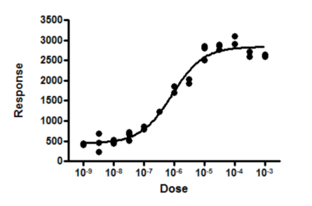
The response at the last two doses dips down a bit. Is this coincidence? Or evidence of a biphasic response?
One way to approach this problem is to specify an alternative model, and then compare the sums-of-squares of the two fits. In this example, it may not be clear which biphasic model to use as the alternative model. And there probably is no point in doing serious investigation of a biphasic model in this example, without first collecting data at higher doses.
Since replicate values were obtained at each dose, the scatter among those replicates lets us assess whether the curve is ‘too far’ from the points.
After checking the option (on the Diagnostics tab) to perform the replicates test, Prism reports these results:
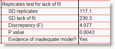
The value in the first row quantifies the scatter of replicates, essentially pooling the standard deviations at all X values into one value. This value is based only on variation among replicates. It can be computed without any curve fitting. If the replicates vary wildly, this will be a high value. If the replicates are all very consistent, this value will be low.
The value in the second row quantifies how close the curve comes to the mean of the replicates. If the curve comes close the the mean of the replicates, the value will be low. If the curve is far from some of those means, the value will be high.
The third row (F) is the square of the ratio of those two SD values.
If the model is correct, and all the scatter is Gaussian random variation around the model, then the two SD values will probably be similar, so F should be near 1. In this example, F is greater than 1 because the SD for lack of fit is so much greater than the SD of replicates. The P value answers this question:
If the model was chosen correctly and all scatter is Gaussian, what is the chance of finding a F ratio so much greater than 1.0?
A small P value is evidence that the data actually follow a model that is different than the model that you chose. In this example, this suggests that maybe some sort of biphasic dose-response model is correct -- that the dip of those last few points is not just coincidence.
How the replicates test calculations are done
This test for lack of fit is discussed in detail in advanced texts of linear regression (1,2) and briefly mentioned in texts of nonlinear regression (3, 4). Here is a brief explanation of the method:
The SD of replicates is computed by summing the square of the distance of each replicate from the mean of that set of replicates. Divide that sum by its degrees of freedom (the total number of points minus the number of X values), and take the square root. This value is based only on variation among replicates. It can be computed without any curve fitting.
The SD lack of fit is a bit trickier to understand. Replace each replicate with the mean of its set of replicates. Then compute the sum of square of the distance of those points from the curve. If there are triplicate values, then each of the three replicate values is replaced by the mean of those three values, the distance between that mean and the curve is squared, and that square is entered into the sum three times (one for each of the replicates). Now divide that sum of squares by its degree of freedom (number of points minus number of parameters minus number of X values), and take the square root.
The F ratio is the square of the ratio of the two SDs.
The P value is computed from the F ratio and the two degree of freedom values, defined above.
References
1.Applied Regression Analysis, N Draper and H Smith, Wiley Interscience, 3rd edition, 1998 page 47-56.
2.Applied Linear Statistical Models by M Kutner, C Nachtsheim, J Neter, W Li, Irwin/McGraw-Hill; 5th edition (September 26, 2004), pages 119-127
3.Nonlinear Regression Analysis & its applications, DM Bates and DG Watts, Wiley Interscience, 1988, pages 29-30.
4.Nonlinear Regression, CAF Seber and CJ Wild, Wiley Interscience, 2003, pages 30-32.