The basic idea of nonlinear regression
You won't be able to understand the mathematical details of nonlinear regression unless you first master matrix algebra. But the basic idea is pretty easy to understand. Every nonlinear regression method follows these steps:
1. Start with initial estimated values for each parameter in the equation.
2. Generate the curve defined by the initial values. Calculate the sum-of-squares -- the sum of the squares of the vertical distances of the points from the curve. (Or compute the weighted sum-of-squares if you are including weighting factors.)
3. Adjust the parameters to make the curve come closer to the data points -- to reduce the sum-of-squares. There are several algorithms for adjusting the parameters, as explained below.
4. Adjust the parameters again so that the curve comes even closer to the points. Repeat.
5. Stop the calculations when the adjustments make virtually no difference in the sum-of-squares.
6. Report the best-fit results. The precise values you obtain will depend in part on the initial values chosen in step 1 and the stopping criteria of step 5. This means that repeat analyses of the same data will not always give exactly the same results.
The Marquardt method
Step 3 is the only difficult one. Prism (and most other nonlinear regression programs) uses the method of Marquardt and Levenberg, which blends two other methods, the method of linear descent and the method of Gauss-Newton. The best way to understand these methods is to follow an example. Here are some data to be fit to a typical binding curve (rectangular hyperbola).
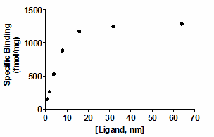
You want to fit a binding curve to determine Bmax and Kd using the equation

How can you find the values of Bmax and Kd that fit the data best? You can generate an infinite number of curves by varying Bmax and Kd. For each of the generated curves, you can compute the sum-of-squares to assess how well that curve fits the data. The following graph illustrates the situation.
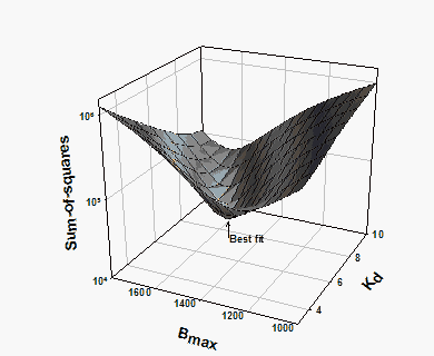
The X- and Y-axes correspond to two parameters to be fit by nonlinear regression (Bmax and Kd in this example). The Z-axis is the sum-of-squares. Each point on the surface corresponds to one possible curve. The goal of nonlinear regression is to find the values of Bmax and Kd that make the sum-of-squares as small as possible (to find the bottom of the valley).
The method of linear descent follows a very simple strategy. Starting from the initial values, try increasing each parameter a small amount. If the sum-of-squares goes down, continue. If the sum-of-squares goes up, go back and decrease the value of the parameter instead. You've taken a step down the surface. Repeat many times. Each step will usually reduce the sum-of-squares. If the sum-of-squares goes up instead, the step must have been so large that you went past the bottom and back up the other side. If this happens, go back and take a smaller step. After repeating these steps many times, you will reach the bottom.
The Gauss-Newton method is a bit harder to understand. As with the method of linear descent, start by computing how much the sum-of-squares changes when you make a small change in the value of each parameter. This tells you the slope of the sum-of-squares surface at the point defined by the initial values. If the equation really is linear, this is enough information to determine the shape of the entire sum-of-squares surface, and thus calculate the best-fit values of Bmax and Kd in one step. With a linear equation, knowing the slope at one point tells you everything you need to know about the surface, and you can find the minimum in one step. With nonlinear equations, the Gauss-Newton method won't find the best-fit values in one step, but that step usually improves the fit. After repeating many iterations, you reach the bottom.
This method of linear descent tends to work well for early iterations, but works slowly when it gets close to the best-fit values (and the surface is nearly flat). In contrast, the Gauss-Newton method tends to work badly in early iterations, but works very well in later iterations. The two methods are blended in the method of Marquardt (also called the Levenberg-Marquardt method). It uses the method of linear descent in early iterations and then gradually switches to the Gauss-Newton approach.
Prism, like most programs, uses the Marquardt method for performing nonlinear regression. The method is pretty standard. The only variations are what value to use for lambda (which determines step size) and how to change lambda with successive iterations. We follow the recommendations of Numerical Recipes. Lambda is initialized to 0.001. It is decreased by a factor of 10 after a successful iteration and increased by a factor of 10 after an unsuccessful iteration.
References
Chapter 15 of Numerical Recipes in C, Second Edition, WH Press, et. Al. , Cambridge Press, 1992
Chapter 10 of Primer of Applied Regression and Analysis of Variance by SA Glantz and BK Slinker, McGraw-Hill, 1990.