1. Create the data table

From the Welcome or New Table dialog, choose to create an XY data table, choose to use tutorial data, and select the sample data "Dose-response: EC50 shift by global fitting" in the set of pharmacology tutorials.

2. Inspect the data

The sample data may be partly covered by a floating note explaining how to fit the data (for people who are not reading this help page). You can move the floating note out of the way, or minimize it.

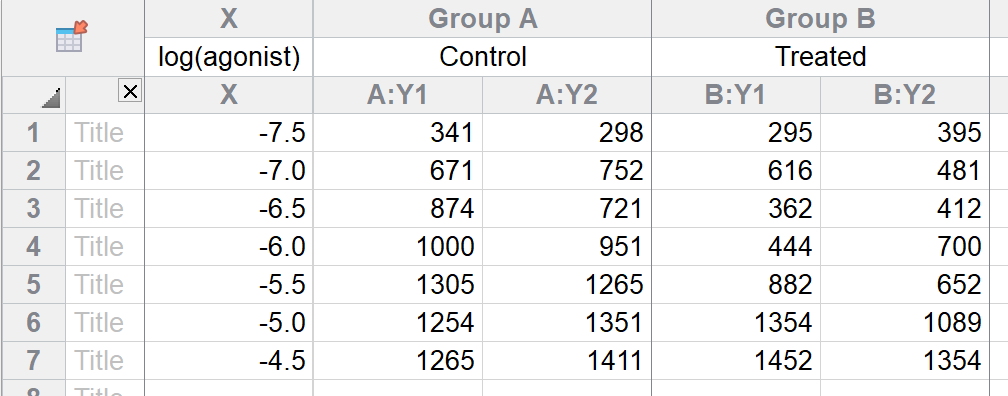
The X values are the logarithm of the concentration of agonist.  Note that "1e-9" is exactly the same as 0.000000001. To enter as a logarithm, enter " -9".

The Y values are responses, in duplicate, in two conditions.

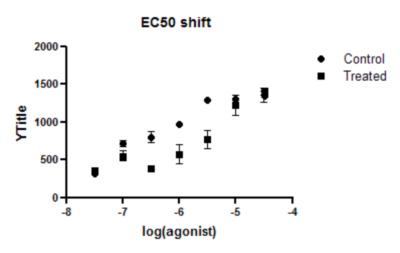
3. View the graph

Since this is the first time you are viewing the graph, Prism will pop up the Change Graph Type dialog. Select the first choice, to plot mean and error bars, and choose SD error bars.

4. Choose nonlinear regression

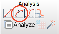
Click and choose Nonlinear regression from the list of XY analyses.

Alternatively, click the shortcut button for nonlinear regression.

5. Choose a model

On the Fit tab of the nonlinear regression dialog, go to the dose-response-stimulation models and choose: log(agonist) vs. response -- variable slope.

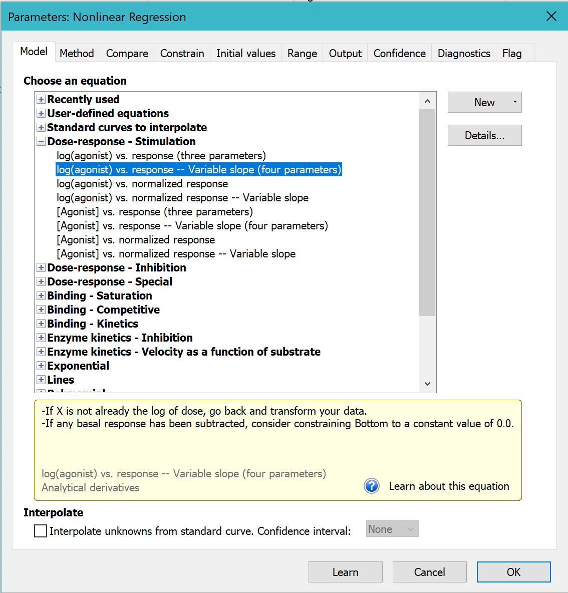
For now, leave all the other settings to their default values.

Click OK to see the curves superimposed on the graph.

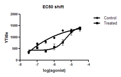
6. Inspect the results

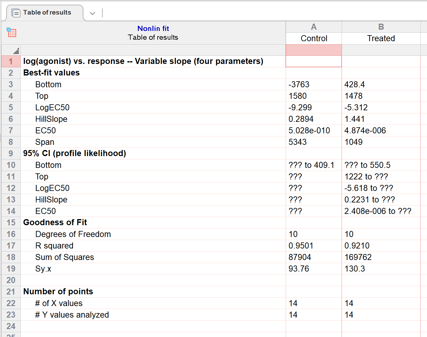
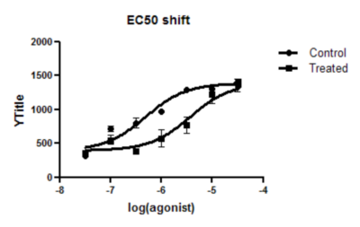
In the results for "Control", it can be seen that - while some best fit estimates were determined - it was not possible to calculate 95% confidence intervals. The situation is slightly better for the "Treated" results, as for each of the best-fit estimates, either an upper- or lower-confidence limit could be calculated (however, none of the best fit estimates have a complete calculated 95% confidence interval). These results should thus only be interpreted with extreme caution.

The reason Prism is unable to calculate complete 95% confidence intervals for these best-fit parameters is that the data do not define the curve well (for example, the control (circles) data set does not define the bottom plateau for the curve). The EC50 is the concentration that gives a response half way between the bottom and top plateaus of the curve. If the bottom cannot be defined accurately, neither can the EC50.

7. Go back to the dialog, and share three parameters

You can get much better results from this data set if you are willing to assume that that the top and bottom plateaus, and the slope, are the same under control and treated conditions. In other words, you assume that the treatment shifts the EC50 but doesn't change the basal response, the maximum response, or the Hill slope.

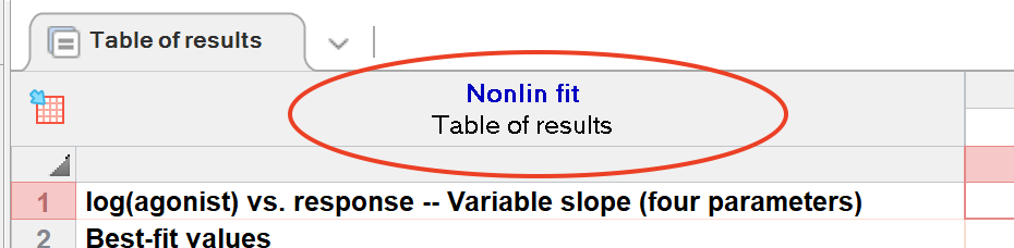
Return to the nonlinear regression dialog by clicking the button in the upper left of the results table.

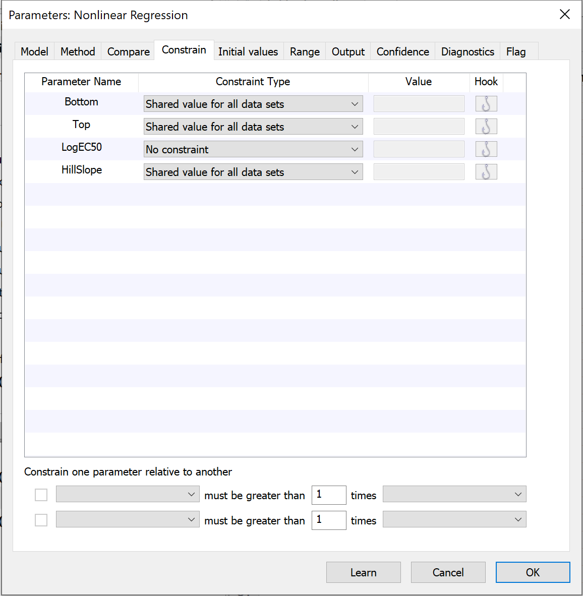
Go to the constraints tab and choose to share the value of Bottom, Top, and HillSlope. When you share these parameters, Prism fits the data sets globally to find one best-fit value for Bottom, Top and HillSlope (for both data sets) and separate best-fit values for the logEC50.

8. View the revised graph and results

 

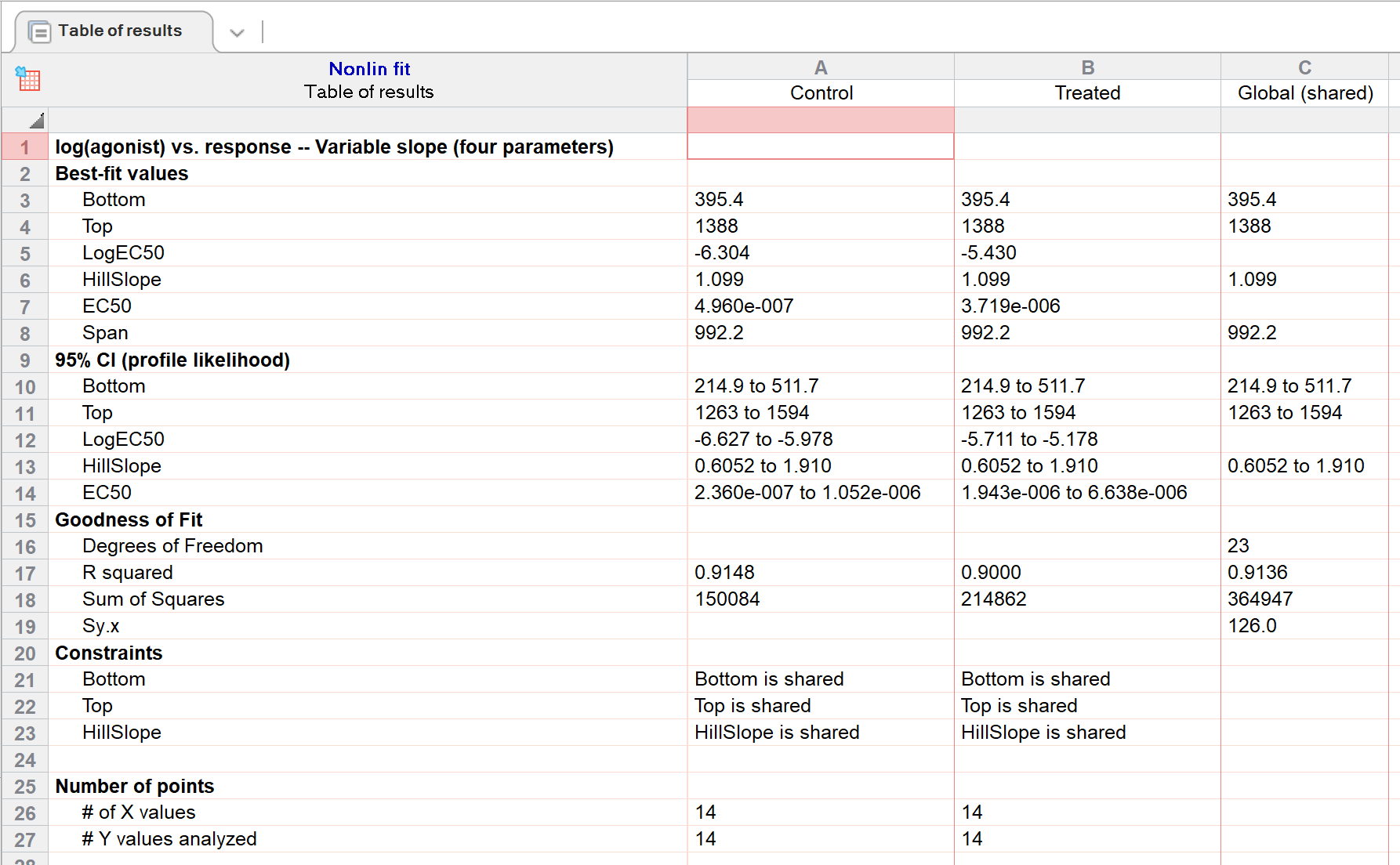
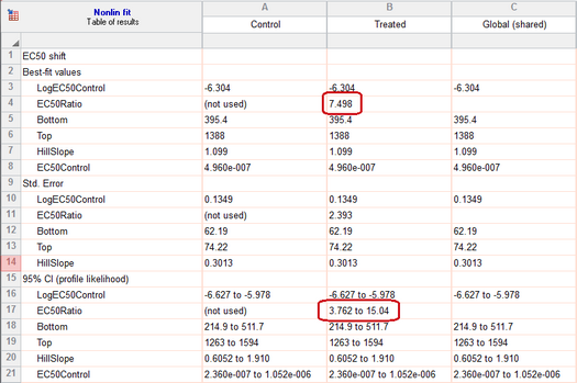
Using this method of parameter sharing, the confidence intervals are much tighter.

9. Statistically compare the two logEC50 values

Go back to the parameters dialog for nonlinear regression and go to the Compare tab. Select the option to test if the selected unshared parameters differ between data sets. Make sure that "Extra sum-of-squares F test" is selected, and then check the box beside "LogEC50".

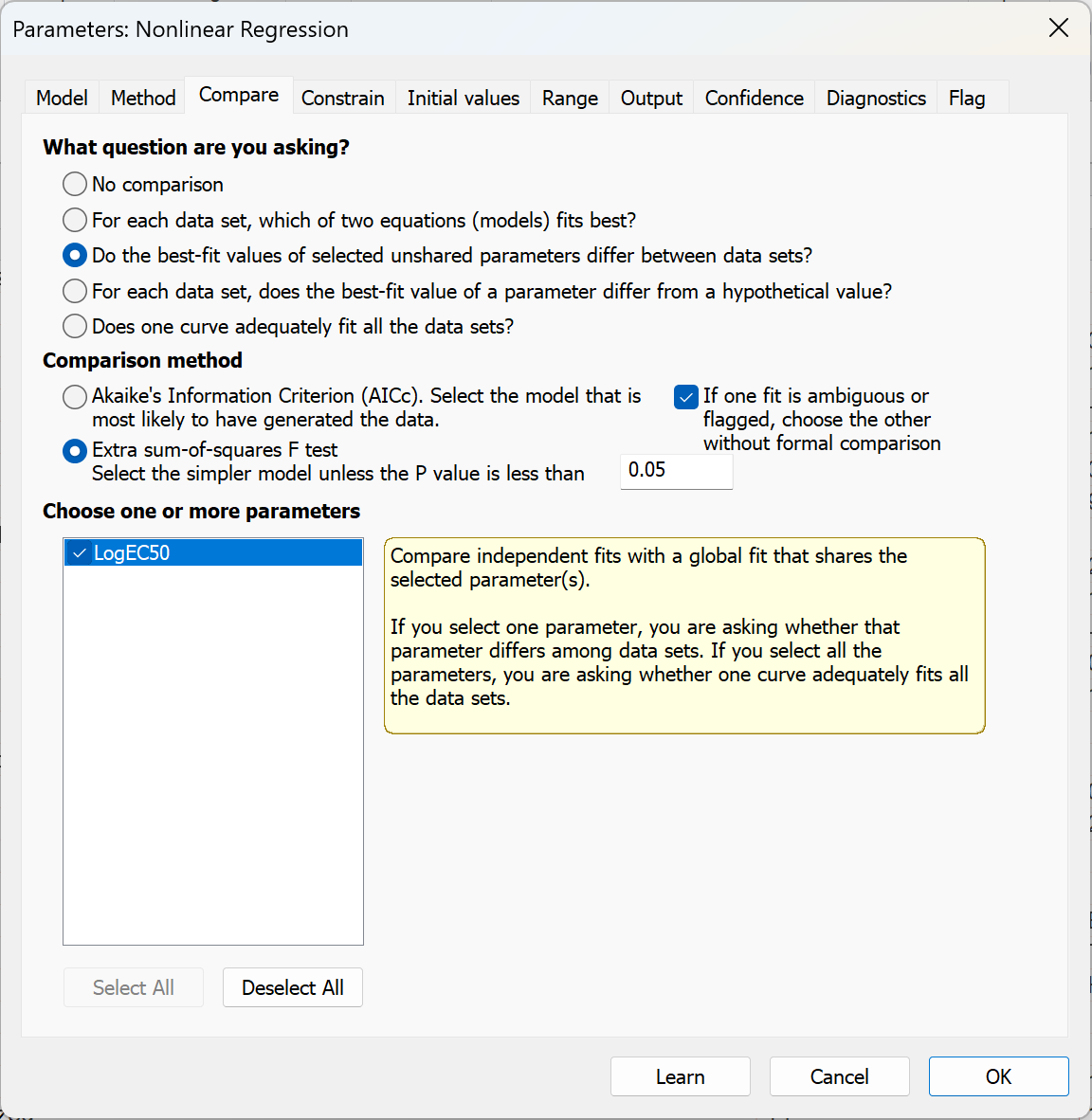
Prism will now fit the data two ways:

1.Fitting models with separate LogEC50 parameters for each data set. This is the same as the fit in the previous step, and will continue to share the "Top", "Bottom", and "Hillslope" parameters as defined in the Constrain tab of the analysis dialog.

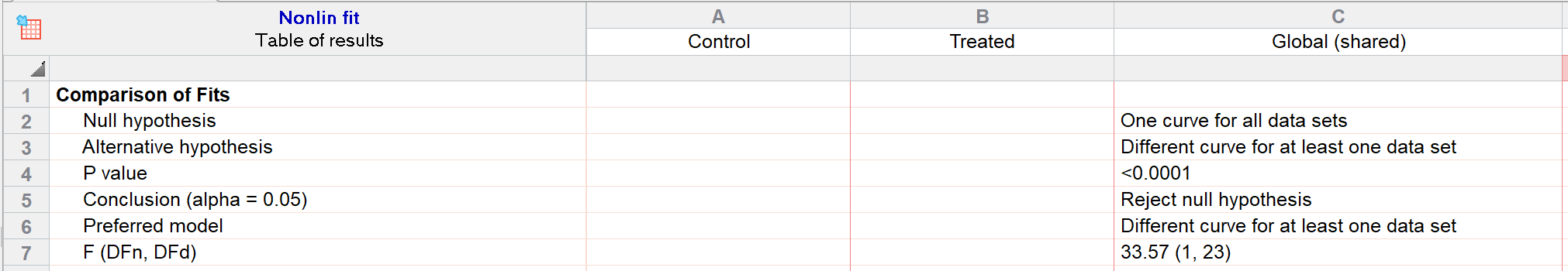
2.Sharing all of the parameters including LogEC50. As with the first method, three of the model parameters were already shared. Since all four parameters are shared in this second fit, Prism fits one curve through all the data, ignoring which treatment group they are in. It compares the sum-of-squares (really the sum-of-sum-of squares since there are two data sets fit in each case), using the extra sum-of-squares F test. The results are shown at the top of the results sheet.

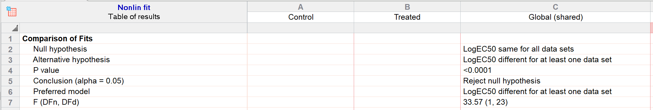
The P value is tiny, so we reject the null hypothesis that the two LogEC50 values are identical in the population, and instead conclude that the two LogEC50 values are different.

Note that because all of the parameters were shared, you could have selected the option "Does one curve adequately fit all the data sets?" on the Compare tab of the analysis parameters dialog. In this case, these two comparison methods would be equivalent (again because all parameters are being shared), and the results of the comparison would be the same (though the phrasing in the results table would be slightly different):

10. Fit the ratio of two IC50 values directly

From the results in step 8, you can compute what you want to know -- the ratio of the two EC50 values.

But Prism can calculate this value directly.

Go back to the analysis parameters dialog, and on the Fit tab, change the equation to "EC50 shift" from the "Dose-response - Special" group of equations. Accept all defaults and click OK. The graph will look identical, as the model is equivalent. But now, rather than fitting two logEC50 values, Prism fits one and also fits the ratio.

This equation was designed to do exactly what is needed for this example. Read about how this equation was set up, so you can construct your own equations when necessary.