Review of how the logistic model is fit

The process of fitting a logistic regression model to a set of data involves identifying a set of “best-fit” values for the parameters of the model. The way this works is by using an iterative algorithm to maximize the likelihood function for the logistic regression model. One way to think about this process is that it’s trying to discover the values of the parameters for the model that were “most likely” to have created the observed data. This results in a couple of important concepts. First, this means that - in general - logistic regression models will perform better at fitting (or classifying) the entered data than they will at correctly predicting outcomes of new data.

The other implication of using this method is that there are some cases in which it is impossible for the algorithm to determine the parameter values, and thus it is impossible in these cases to define a logistic regression model. Three common cases with logistic regression in which this occurs include: perfect separation, quasi-perfect separation, and linear dependence of X variables.

Perfect separation

Perfect separation, sometimes also referred to as complete separation, is the term that is used when a model that predicts the data perfectly. Another way of stating this is that for a given predictor (or some linear combination of predictors), one outcome always occurs above a certain value of the predictor, while the other outcome always occurs below that value. That might sound a bit confusing, but in practice what it means is that the model would correctly classify every point entered as a 0 as a negative outcome and every point entered as a 1 as a positive outcome. On the surface, this doesn’t seem like a major problem as one of the goals of logistic regression is to classify the observed outcomes. However, another goal of logistic regression is to find the best-fit estimates of the model parameters, The problem with perfect separation is that, in these situations, there is no single set of best fit values that maximize the likelihood. Let’s look at a simple example:

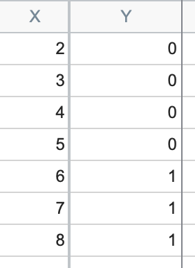
You can see that for every value of X equal or less than 5, the Y value is 0. And for every value of X greater than 5, the Y value is 1. When there’s only one predictor (such as with simple logistic regression), we can see what perfect separation means graphically:

It’s clear that a vertical line can be drawn between X=5 and X=6 for which all points to the left of the line are at Y=0 and all points to the right of the line are at Y=1. So it is easy to predict the outcome from X. But the S shaped logistic curve can't do that job, because the data give no clue as to where that curve should be between 5 and 6. If X=5.5, what is the predicted probability?

Quasi-perfect separation

Quasi-perfect separation is a closely related issue to perfect separation. It occurs when a predictor (or linear combination of predictors) classifies the outcome correctly except at a single value or point. Again, let’s look at some data to better understand this issue:

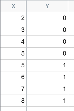
You can see now that for all values of X less than 5, the Y value is 0. And for all values of X greater than 5, the Y value is 1. However, AT X=5, we have both Y=0 AND Y=1. Once again, the likelihood cannot be maximized, so best-fit estimates of the parameters cannot be determined.

Finally, if all of your X values are the same value, it will be impossible for Prism to fit a logistic model to the data or to maximize the likelihood function (see section below describing linearly dependent X variables).

Keep in mind, however, that if you're getting this error, it doesn’t necessarily represent a problem in your experimental design or your data. It could simply mean that you have identified the X variable (or variables) that are capable of perfectly (or quasi-perfectly) predicting your outcome!

Linearly dependent X variables

Another possible problem when attempting to fit a logistic model to your data is the presence of linearly dependent X variables. When a model contains linearly dependent predictors, the algorithm to fit the model will fail because the maximum of the likelihood function won’t exist. To understand this, let’s first define what linearly dependent means. If any of your X variables can be expressed as a linear combination of other variables, then your variables are said to have linear dependence. That didn’t help much unless we also define what a linear combination of variables means. A linear combination of variables refers to the sum of a given set of variables, each multiplied by a constant. This is probably explained easiest via an example. Let’s say you have three variables: X1, X2, and X3. Now, we’ll write a formula:

X3 = A*X1 + B*X2

If there are any values of A and B that could make that expression true, then X3 is a linear combination of X1 and X2. Let’s look at some data to make this concept even more clear:

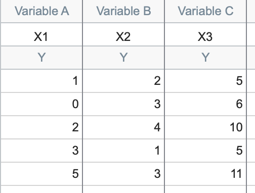
This data shows our three variables (the variables could be anything: age, height, number of steps taken to get to the bathroom…). For this data, the linear relationship is fairly easy to spot:

X3 = 1*X1 + 2*X2

In other words, in every row, the third value is the sum of the first value plus twice the second value. Other linear relationships might not be so easy to spot:

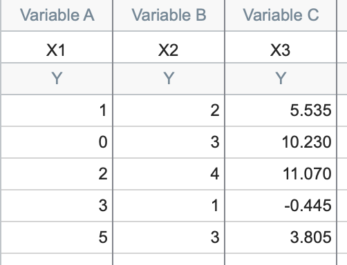
The values in the first two columns are the same, but here the linear relationship is given by:

X3 = -1.285*X1 + 3.41*X2

Another way that the linear dependence issue can present itself is if you have duplicated X columns. This may happen unintentionally when using categorical predictors that have been coded. Coded categorical predictors can only take on a limited number of values, and so it’s easy to see how two otherwise unrelated categorical variables could happen to end up with the same values for each observation (this is even more possible with variables that are in some way related). Of course, the odds of this happening by chance decrease with an increasing number of observations.

One easy to understand example of two variables that would be identical could be from the analysis of football (soccer) games. Imagine that one variable was used and represented “goals made”, while a second variable could be “final score”. It seems obvious in this case, but you should always be wary of duplicate (or linearly dependent) variables that are disguised as independent variables in your model.

If you have duplicated X columns, X columns that are perfectly correlated, or X columns that have a more complicated linear relationship, then the optimization algorithm will fail. To evaluate this problem, use the multicollinearity option in the multiple logistic regression dialog. See the multicollinearity page for more details.

Summary of (some) potential problems with Logistic Regression Model Convergence

1.You have too few 0s or 1s (we recommend, if possible, at least 10 rows of each for each independent (X) variable)

a.In the extreme case, if you have all 0s (or all 1s), you are guaranteed perfect separation, since there is no way for the algorithm to distinguish between the two outcomes.

b.Another extreme case is if you have as many or more X variables as rows of data. There is no way to estimate model error in this case.

2.One of your X variables (or a linear combination of X variables) results in perfect separation or quasi-perfect separation of your Y variable.

3.Your X variables exhibit linear dependence.