To give you a sense of how mathematical models work, below is a brief description of three commonly used models.

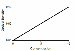
Optical density as a function of concentration

Background

Colorimetric chemical assays are based on a simple principle. Add appropriate reactants to your samples to initiate a chemical reaction whose product is colored. When you terminate the reaction, the concentration of colored product is proportional to the initial concentration of the substance you want to assay.

Model

Since optical density is proportional to the concentration of colored substances, the optical density will also be proportional to the concentration of the substance you are assaying.

Reality check

Mathematically, the equation works for any value of X. However, the results only make sense with certain values.

•Negative X values are meaningless, as concentrations cannot be negative.

•The model may fail at high concentrations of substance where the reaction is no longer limited by the concentration of substance.

•The model may also fail at high concentrations if the solution becomes so dark (the optical density is so high) that little light reaches the detector. At that point, the noise of the instrument may exceed the signal.

It is not unusual for a model to work only for a certain range of values. You just have to be aware of the limitations, and not try to use the model outside of its useful range.

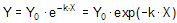
Exponential decay

Exponential equations whenever the rate at which something happens is proportional to the amount which is left. Examples include ligands dissociating from receptors, decay of radioactive isotopes, and metabolism of drugs. Expressed as a differential equation:

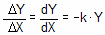
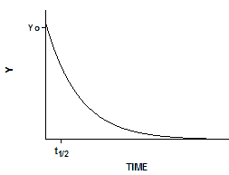
Converting the differential equation into a model that defines Y at various times requires some calculus. There is only one function whose derivative is proportional to Y, the exponential function. Integrate both sides of the equation to obtain a new exponential equation that defines Y as a function of X (time), the rate constant k, and the value of Y at time zero, Y0.

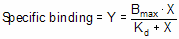
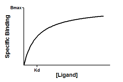
Equilibrium binding

When a ligand interacts with a receptor, or when a substrate interacts with an enzyme, the binding follows the law of mass action.

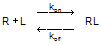
You measure the amount of binding, which is the concentration of the RL complex, so plot that  on the Y axis. You vary the amount of added ligand, which we can assume is identical to the concentration of free ligand, L, so that forms the X axis. Some simple (but tedious) algebra leads to this equation: