After performing Cox proportional hazards regression, it may be of interest to investigate how well the model performs at describing the input data. One way to assess this goodness of fit is to compare the hazards for each individual that are estimated by the model and the observed survival times in the input data for these same individuals.
Short version
Prism reports a value for Harrell's C (concordance) statistic and its associated 95% confidence interval. To calculate the C statistic, all possible pairs of observations where at least one of the pair includes an event are considered (pairs where both observations are censored are omitted from the calculation). For each pair, the observation time ("T", entered in the table) and the relative risk ("XB", determined by the model) are compared. Pairs in which the observation with the shorter time to event is also the observation with the higher relative risk are considered "concordant" (these are pairs of observations in which the model correctly identified the observation that should have a shorter survival time by assigning it a higher relative risk). Pairs that don't fit this expected relationship are considered "Discordant" (or in some cases, simply cannot be identified as "concordant" because they have tied values in either their observed time or relative risk scores, see the "Detailed version below).
The C statistic represents the proportion of concordant pairs (the fraction of pairs in which the model correctly predicted a shorter survival time), and thus takes on a value between 0 and 1. This value is a conditional probability that - for any pair of observations - the model assigns a higher hazard ratio to the observation with the shorter survival time. Thus, models with a C statistic close to 1 suggest that the model has better discrimination capabilities, while models with C statistics close to 0.5 do no better than random chance. Models with C statistics less than 0.5 are extremely rare and generally only occur as a result of variation in very small sample sizes. If you see a C statistic less than 0.5, something probably went wrong!
Intuition behind C statistic
For a given observation, a larger relative risk (XB) value suggests a higher hazard and thus a shorter survival time. Thus, if one observation has a higher XB value and a lower elapsed time to event than another observation, these observations can be thought of as behaving as expected. However, if an observation has a higher XB value and a longer elapsed time to the event of interest than another observation, then these observations can be thought of as behaving abnormally. Concordance is simply the fraction of data pairs that behave as expected (assuming no ties in relative risk values between any pairs of observations).
Another way to interpret Concordance is to think of the model as a predictive device. When presented with two observations of data, this model will make a prediction about which of the two observations will survive longer. A perfect predictive device will correctly predict every pair of observations, while a truly random device would be expected to predict half of the pairs correctly (think of the model as a device that just flips a coin to decide which observation should have the higher relative risk: we'd expect it to be right ~50% of the time).
The value of concordance reflects this behavior, and must take on a value between zero and one. A value of one means that the model correctly predicted all of the pairs of observations (observations predicted to live longer do live longer, and observations predicted to experience the event of interest sooner do experience it sooner). If the model is truly random, this value of concordance would be 0.5, indicating that half of the time, the model would correctly predict which observations “survives” longer until the event of interest.
If this concept of concordance sounds similar to the goodness-of-fit metric reported by logistic regression of the area under the ROC curve, it’s because these two concepts are absolutely equivalent.
Detailed version
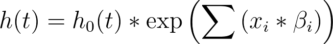
Recall the model for Cox proportional hazards:
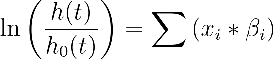
This can be rearranged to the form:
Note that in the context of Cox regression “xi” indicates the value of a predictor variable (like age, weight, treatment group, etc.).
Cox proportional hazards doesn’t actually assume any specific form for the baseline hazard, but it can be seen that the linear predictor (Σxi*βi, or just “XB” for short) is proportional to the hazard rate (h(t)). This means that as the value of XB increases, the hazard rate increases. Subsequently, as the hazard rate increases, the probability of experiencing the event of interest increases, and thus survival time is expected to decrease.
In summary, a larger XB predicts a shorter elapsed time to the event of interest.
Using the calculated parameter coefficients (β) and the observed time to event data in the input data table, we can evaluate how well the model performs at predicting this relationship. This is done via Harrell’s C statistic for concordance.
Popularized by Frank Harrell (1), this value can be interpreted as follows:
•Consider every possible pairwise combination of observations in the input data table in which at least one observation is an event (pairs in which both observations were censored are omitted from the calculation)
If both observations in the pair contain an event
•Compare the linear predictor (XB) determined by the model and the observed time to the event of interest in the input data for each observation
▪For the sake of notation, let’s call the relative risk for the first observation XB1, the relative risk for the second observation XB2, the elapsed time for the first observation T1 and the elapsed time for the second observation T2
•Pairs of observations are considered “concordant” if:
▪XB1 > XB2 and T1 < T2
▪XB2 < XB2 and T1 > T2
•Pairs of observations are considered “discordant” if:
▪XB1 > XB2 and T1 > T2
▪XB1 < XB2 and T1 < T2
•Pairs of observations are considered "tied in XB" if:
▪XB1 = XB2
•Pairs of observations are considered "tied in T" if:
▪T1 = T2
•Pairs of observations are considered "tied in XB and T" if:
▪XB1 = XB2 and T1 = T2
If one observation in the pair is censored
•For the following definitions the observation with the event will have observation time Te and relative risk XBe while the observation that was censored will have observation time Tc and relative risk XBc
•If Tc < Te, then we can't know for sure who experienced the event first (the individual with the censored observation left before the event occurred), and so this pair of observations is omitted from the calculation
•The pair of observations is considered "concordant" if:
▪Tc ≥ Te and XBc < XBe
•The pair of observations is considered "discordant" if:
▪Tc ≥ Te and XBc > XBe
•The pair of observations is considered "tied in XB" if:
▪XBc = XBe
•Pairs of observations with one censored and one event cannot be tied in T
Formula for Concordance statistic
Using the definitions above, determine the following:
•nconcordant, the number of concordant pairs
•ndiscordant, the number of discordant pairs
•ntied in XB, the number of pairs tied in XB
When there are no ties in XB for any pair of observations, the formula for the C statistic is given as:
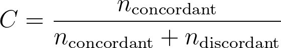
This represents the "fraction" of observations that the model was able to correctly assign an appropriate relative risk value to (higher relative risk values should result in lower survival times). If - for all pairs of observations - the observation with the larger relative risk is also the observation with the shorter survival time, then all pairs would be concordant, and this fraction would be equal to 1! When there are pairs of observations with ties in their relative risk values, the formula is slightly different:
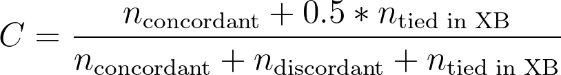
This formula is similar, but adds a term for the tied observations in both the numerator and the denominator. Going back to the “predictive device” example from the earlier section, we can consider what happens when the model is presented with observations that are tied in the linear predictor (XB). In this situation, the predictive device can’t know which observation should survive longer, and so all it can do is flip a coin to make a decision. We would expect the coin flip to be correct about 50% of the time, which is why the number of observation pairs tied in XB is multiplied by 0.5 in the numerator of the above equation. Thus, in this case, the C statistic still represents the fraction of observations that the model was able to correctly assign an appropriate relative risk value.
References
1.Harrell FE, Califf RM, Pryor DB, Lee KL, Rosati RA. Evaluating the yield of medical tests. Journal of the American Medical Association. 1982;247:2543–46.