What does the "power" of a test actually mean?

When performing an experiment, you're typically interested in measuring some effect: are the protein concentrations in the drug-treated group different from the control group; is the median survival time longer in the knock-out strain compared to the wild-type; is the gene expression different between the different treatment groups?

Your experiment uses samples from different populations to gather data and perform your statistical analyses. The idea is that if the effect that you're looking for truly exists in the populations then you would (hopefully) observe it in your samples. However, there is variability within populations, and you can't always be certain that the samples that you've selected from the broader populations will allow you to detect your target effect.

In simplified terms, analyses using classic hypothesis testing approaches start with a null hypothesis that there is no effect, and an alternative hypothesis that there is an effect. In the scenario above, we assume that the effect DOES exist in the population. But by chance alone, data generated from the samples you selected did not reflect that effect. In other words, your data may yield a P value greater than 0.05 (or whatever value of alpha you've used as your statistical threshold). Because of this, you would not reject the null hypothesis (that there is no effect) even though the effect DOES exist in the populations you sampled from!

The "power" of a test is the probability that you will reject the null hypothesis when it is false. Another way to say this is that power is the probability that you reject the null hypothesis when the effect that you're looking for exists in the population. Think again about our example: we started by stating that the effect does exist in the populations, but due to variability in the populations and randomly sampling from those populations, we may or may not be able to observe the effect. Power tells us what the probability of observing the effect is, and depends on many factors including the size of the effect in the population, the size of the samples that we're drawing from the population, and the variability within the populations.

Another way to think about power: running infinite experiments

Let's assume we are comparing two means with a t test, and that the means of the two populations truly do differ by a particular amount. We start by collecting samples from the two populations of interest, measure the sample means, perform our t test, and get a P value. Because of the variability in the populations that we sampled from, this P value may be greater than alpha (usually 0.05) or it may be less than alpha.

But now let's assume that we pick new samples from the populations and run the test again. Because of the variability and sampling, the sample values will be slightly different, and the t test will yield different results. We'll get a different P value from this new test which (again) may be greater or less than alpha.

Now let's assume that we keep doing this process over and over. Some of the calculated P values will be less than alpha and we will reject the null hypothesis, while other calculated P values will be greater than alpha and we won't reject the null hypothesis. We started by stating that there is a difference in the population means, so if we run the same experiment (with the same sized samples drawn from the same populations), then we would obtain a certain percentage of experiments where the P value is less than our threshold. If the experiment was repeated an infinite number of times, then the percentage of experiments where the P value was less than the threshold would be the power of the experiment.

Take note that this can't be done in real life for a couple of reasons:

1.We don't have the time or resources to perform an infinite number of experiments

2.More importantly, we don't know if the effect truly exists in the populations that we're sampling from. If we already knew that there was an effect, then there wouldn't be much of a point in running these experiments!

More technical definitions of power (and beta)

Typically when you draw a sample from a population, your objective is to determine some statistic from it (a mean, a standard deviation, etc.). Another type of statistic might be the difference between two sample means. Yet another statistic might be that difference between sample means divided by the pooled standard deviation for the two samples. This last statistic is actually the t statistic used in a t test.

Regardless of the statistic that you're calculating, there will be a range of possible values for that statistic due to the fact that you drew a sample from a larger population, and that population has variability. If you draw many different samples, you're almost certainly going to get many different statistic values. The distribution of values that this statistic can take is given by something called a "sampling distribution". When looking at statistics to determine if a predicted effect exists between different populations, the distribution of possible values for the statistic also greatly depends on whether or not that effect truly exists.

Fortunately, with enough information about the populations and the predicted effect, it's possible to construct sampling distributions for statistics assuming that the effect does exist AND assuming that it doesn't. Let's look at an example for a t statistic:

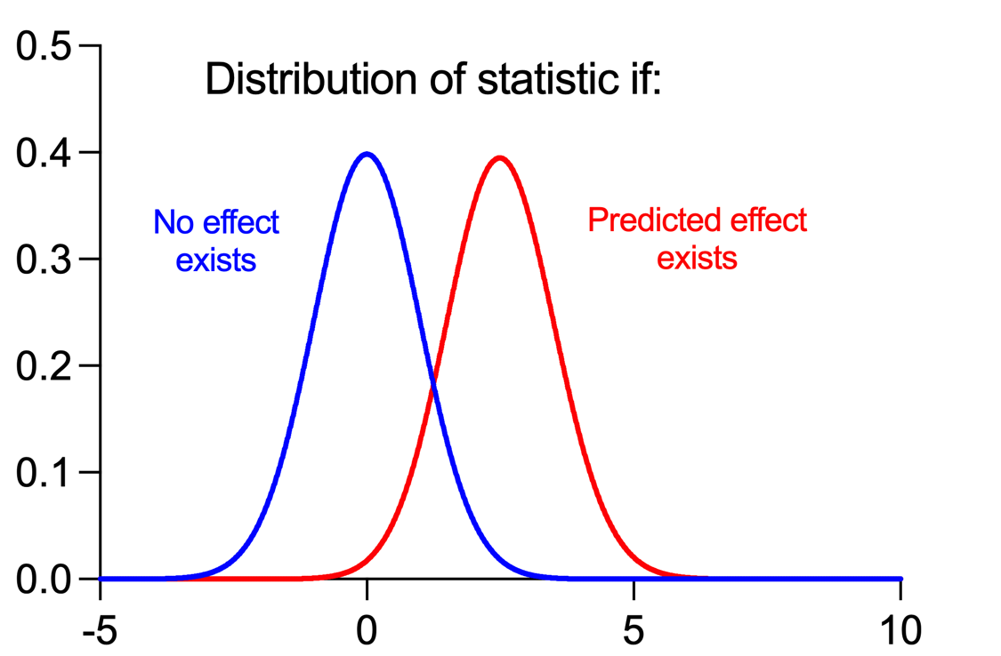
The blue curve is the sampling distribution assuming that no effect exists. Note that the distribution is centered at zero, which makes sense if there is no effect. However, because of the variability in the populations and the fact that samples are being drawn from them, it's still possible to obtain t statistics that are larger or smaller than zero even when no effect exists.

The red curve is the sampling distribution assuming that a specific predicted effect does exist. In this case, the distribution is centered at approximately 2.5. This is due to the fact that if the predicted effect exists, it's much more probable for the determined t statistic to be farther from zero (but not impossible to be zero).

When you perform an experiment by drawing samples from these populations and calculating a t statistic, you will compare that t statistic to a "critical value" to determine if the results you obtained are statistically significant or not. This can be shown visually using these curves. Here's the sampling distribution for the null hypothesis (blue curve, no effect exists) along with the critical t value (vertical line):

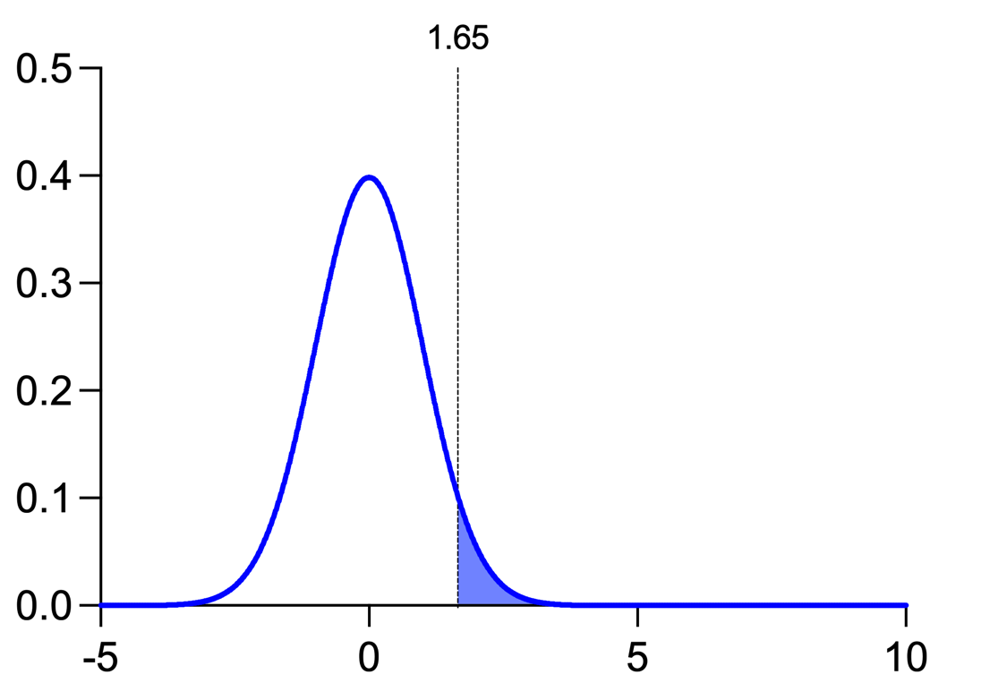
The shaded region represents the probability of getting a t statistic value that is greater than the critical value if the null hypothesis is true. In this case, the shaded region represents 5% of the total area under this curve. This is a representation of the concept of alpha which is the probability of rejecting the null hypothesis when it is actually true. If you used a different alpha, you would obtain a different critical value, and you would end up with a different amount of the curve in the shaded region.

In a similar fashion, the critical value can be used in combination with the red curve:

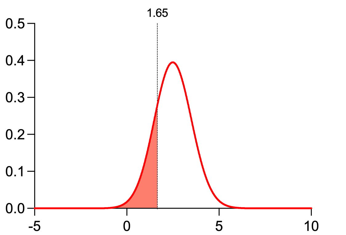
In this case, the shaded region represents the probability of getting a t statistic value that is less than the critical value if the alternative hypothesis is true. Here the shaded region represents 20% of the total area under this curve. This is a representation of the concept of beta, which is the probability of failing to reject the null hypothesis when it's false (a Type II error). In other words, it's the probability of not detecting an effect when it actually exists. You may notice that alpha (probability of making a type I error) is 4x smaller than beta (probability of making a type II error), and these are pretty common values. One way to think about this is that using these values means that avoiding a type I error (a false positive) is 4x more important than a type II error (a false negative).

Power is actually derived directly from beta:

Power = 1 - β

So in the example above where beta is 0.20, power would equal 0.8 or 80%. Like with alpha and a value of 0.05, this is simply a commonly used value for Power, but is not a strict requirement. Ultimately, it's up to you as the researcher to decide what value of power you would like to achieve when designing your experiments. The next section discusses this in a bit more detail.

Putting the images and information from above together, we can get the following:

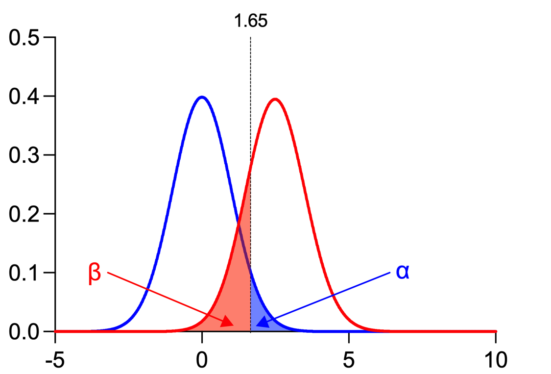
•Alpha (α): Probability of a Type I error (rejecting the null hypothesis when it is true, a "False Positive"), Typically 0.05 or 5%

•Beta (β): Probability of a Type II error (not rejecting the null hypothesis when it is false, a "False Negative"), Typically 0.2 or 20%

•Power (1-β): Probability of rejecting the null hypothesis when it is false (when the effect truly exists), Typically 0.8 or 80%

How much power do I need?

The power is the chance that an experiment will result in a "statistically significant" result from your samples assuming that the investigated effect truly exists in the populations sampled. How much power do you need? These guidelines might be useful:

•If the power of a test for an experiment is less than 50%, then you'll only detect the target effect if it exists in half of your experiments. A study with this amount of power is really not very helpful, and (potentially worse) unlikely to be reproducible

•Many investigators choose sample size to obtain a 80% power. This is arbitrary, but commonly used

•Ideally, your choice of acceptable power should depend on the consequence of making a Type II error.

Power Analysis with Prism

Power Analysis (and sample size calculations) can be performed for various experimental designs via Prism Cloud.