The Residuals tab of the Cox proportional hazards regression parameters dialog is used to generate a number of different graphs that provide insight into the quality of the model fit, and assess the validity of some of the assumptions made as part of the analysis.
It is important to note that the values referred to in Cox regression as residuals are not residuals in the classic sense. In multiple linear regression (as well as simple linear regression and nonlinear regression), a residual is defined as the difference between the observed value of the outcome variable and the predicted value of the outcome variable for the same observation. For example, if a multiple linear regression model was generated to estimate an individual’s height using variables about the individual’s age, gender, and weight, you could compare each of the measured heights used to construct the model, and the corresponding heights predicted by the model using the same input values of age, gender, and weight. The difference between these two values (observed and predicted) is the residual.
Unfortunately, there is no direct analog of this “actual minus observed” concept available for Cox proportional hazards regression. Instead, a number of different values have been proposed that attempt to answer the same questions in Cox proportional hazards regression that standard residuals answer for other types of regression (like multiple linear regression).
Is the proportional hazards assumption valid?
The first of these questions asks if the assumption of proportional hazards is valid. This assumption essentially means that the ratio of hazards for any two individuals in the studied population will be constant over time (see the examples of hazards in this section of the guide). To check the validity of this assumption, Prism offers two graphs: Scaled Schoenfeld residuals vs time or row order, and the Log-minus-log survival plot.
•Scaled Schoenfeld residuals vs. time/row order - if the proportional hazards assumption is valid, these residuals should be randomly distributed about a horizontal line centered at zero. If there is a visible trend in these residuals, the proportional hazards assumption has likely been violated. Note that no scaled Schoenfeld residual is present for censored observations
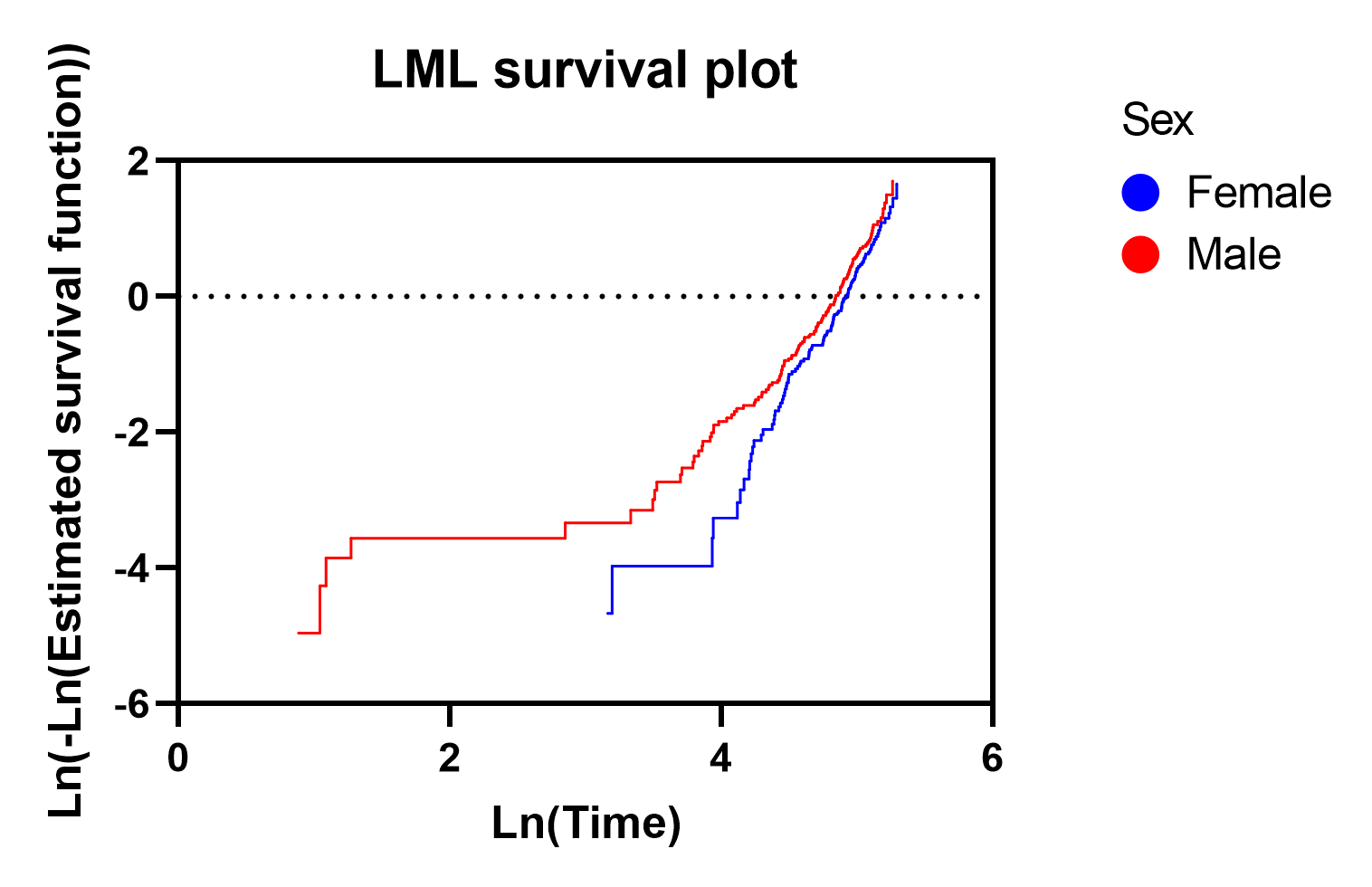
•Log-minus-log (LML) survival plot - if the specified model contains categorical variables, the options for this graph allow you to select these categorical variables to build LML plots for. The graph contains one curve for each group (level) within the selected categorical variable(s). To build these curves, the Nelson-Aalen hazard estimate is used to calculate a cumulative hazard for each group. Recall that cumulative hazard H(t) = -Ln(S(t)). Taking the natural log of this Nelson-Aalen cumulative hazard estimate for each group, we obtain Ln(H(t)) or Ln(-Ln(S(t))). This is the “log-minus-log” value that the graph name refers to, and is plotted on the Y axis with Ln(time) plotted on the X axis. If the proportional hazards assumption is valid, the curves for each group (level) of a single categorical predictor variable will be roughly parallel. The graph below shows a LML plot comparing curves for "Females" and "Males". While the lines in this graph are not perfectly parallel, they suggest that the proportional hazards assumption has not been severely violated for this analysis. If curves for groups (levels) of a single categorical predictor variable cross each other, it’s likely that the proportional hazards assumption of the analysis has been violated.
Note that when creating a LML plot, Prism will also include the un-transformed "Time" and "Estimated survival function" values which can be plotted on the X and Y axes of the graph. For the specified grouping variable(s), the result is a standard nonparametric survival curve for each selected group/level.
Were there outliers in the observations?
A number of different residual graphs for Cox proportional hazards have been proposed in order to detect potential outliers in the input data for the analysis.
•Deviance residuals vs linear predictor/HR - points on this graph should be roughly centered around zero, while points with large absolute values for the residual may represent outliers. Note that trends observed in these graphs may be due to insufficient sample size or patterns in the way observations were censored.
•Martingale residuals vs linear predictor/HR - like deviance residuals, these can be used to find potential outliers in the data. However, these residuals are skewed (not centered about zero), with residuals for event observations in the range of (-inf, 1] and those for censored observations in the range of (-inf, 0]. These residuals are typically harder to interpret than deviance residuals. Note that trends observed in these graphs may be due to insufficient sample size or patterns in the way observations were censored.
•Schoenfeld residuals vs time or row order - unlike deviance and Martingale residuals, these residuals are used to determine the influence of an observation on each of the regression coefficients. When selecting this residual, a graph will be generated that will allow you to examine the Schoenfeld residuals for each different variable coefficient. This graph may also be used to test the proportional hazards assumption (if these graphs exhibit a non-zero slope, the proportional hazards assumption may have been violated)
Are the predictor variables linear?
Prism offers two graphs that can be used to assess the linearity of the effect that the predictor variables have on the model. Like the graphs investigating the potential presence of outliers, either deviance residuals or Martingale residuals can be used.
•Deviance residuals vs covariate - this will generate a graph plotting the deviance residuals against each of the continuous predictor variables in the model. As before, the deviance residuals are expected to be randomly centered around zero. Trends in these residuals may suggest a departure from linearity for the selected predictor variable
•Martingale residuals vs covariate - these residuals are skewed, falling in the range of (-inf, 1], but should still have an average of zero. Visible trends in these residuals may suggest a departure from linearity for the selected predictor variable. These residuals are typically harder to interpret than deviance residuals
How good was the fit?
These residual graphs are only offered as a means of comparing the results generated by Prism with results generated in other statistical packages or those previously published in literature. Cox-Snell residuals were one of the first residuals developed for Cox proportional hazards regression, and have been largely replaced by the other residuals listed on this page.
•Cox-Snell vs Nelson-Aalen estimate of the cumulative hazard rate - this graph was originally suggested for use in assessing a model’s overall fit. A well-fitted regression will generate a nearly straight line of points on this graph that passes through the origin and has a slope of one. However, the problem with this graph is that it would take a particularly ill-fitted model to generate a visualization that doesn’t have this appearance, and it provides no insight into why the fit was poor (violation of proportional hazards assumption, outliers, time-dependent variables, etc.).