1. Create the data table
From the Welcome or New Table dialog, choose to create XY data table, choose to use tutorial data, and select the sample data "Dose-Response - Ambiguous until constrained" from the list of Pharamcology tutorials. Note that this choice is in a drop down menu of sample data sets.
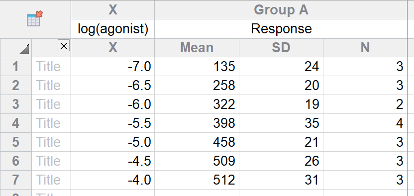
2. Inspect the data table
The X values are the logarithms of molar concentration. The Y values are responses, entered as mean and SD. With Prism, you can either enter replicate values or enter error values (here SD) computed elsewhere.
3. View the graph
Since this is the first time you are viewing the graph, Prism will pop up the Change Graph Type dialog. Select the first choice, to plot mean and error bars, and choose the kind of error bars you prefer.
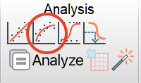
4. Choose nonlinear regression
Click  and choose from the list of XY analyses.
Even faster, click the shortcut button for nonlinear regression.
5. Choose a model
On the Fit tab of the nonlinear regression dialog, open the panel of Stimulatory dose-response equations and choose: log(agonist) vs. response -- Variable slope.
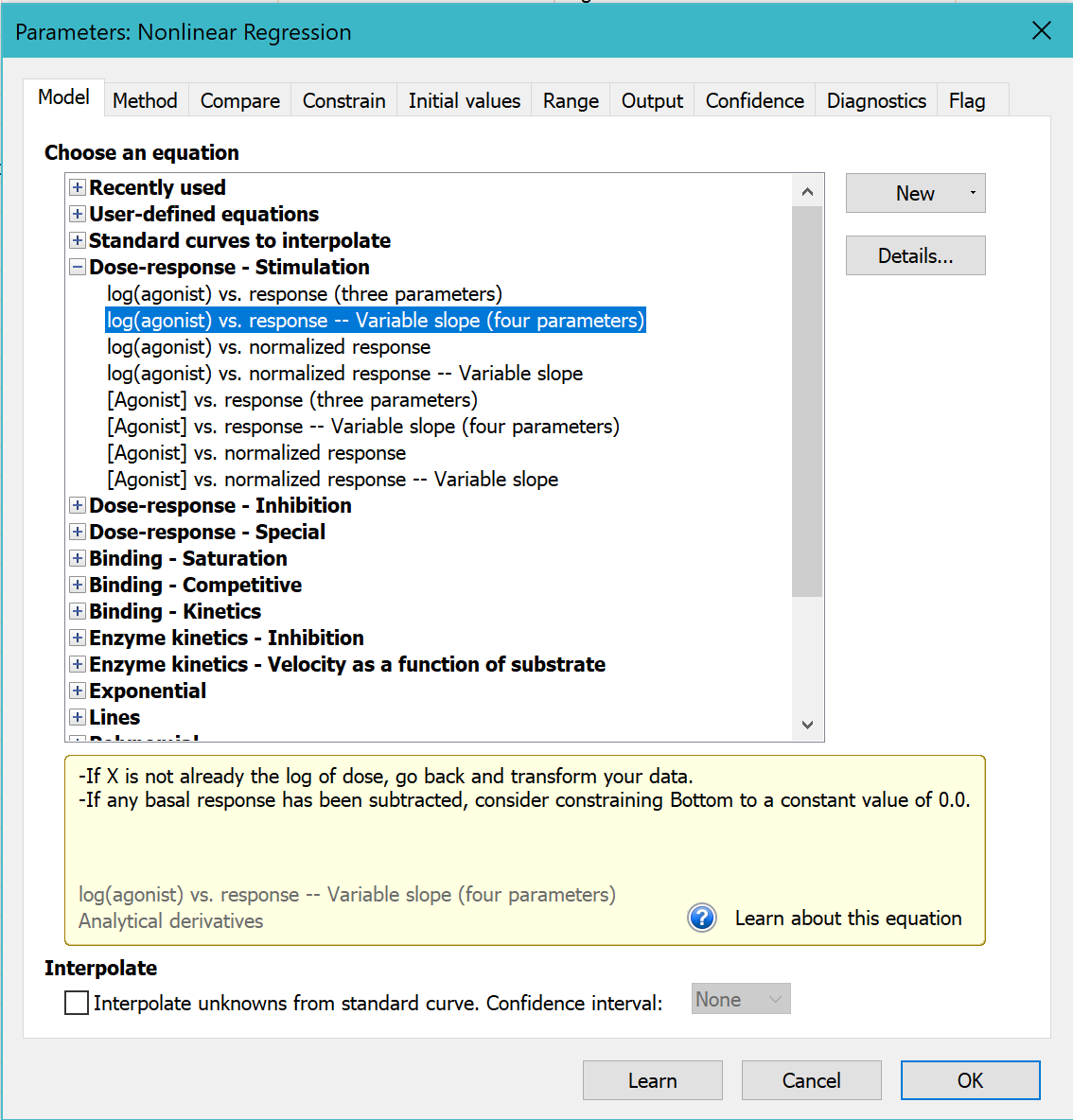
Learn more about fitting dose-response curves.
6. Choose to detect "Ambiguous" model fits
On the Confidence tab of the nonlinear regression dialog, make sure that the option to "Identify "ambiguous" fits" is selected (this is no longer the default option, and we now recommend that you use the "Identify 'unstable' parameters" option instead).
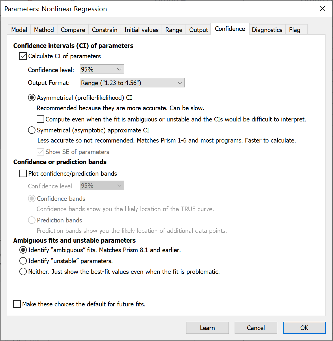
For this example, leave all the other settings to their default values.
Click OK to see the curves superimposed on the graph.
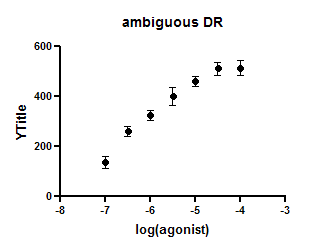
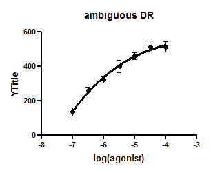
7. Inspect the graph
The curve goes through the point nicely, and looks fine.
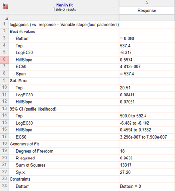
8. Inspect the results
Go to the results page, and view the results.
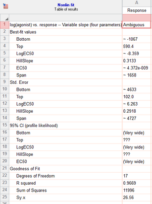
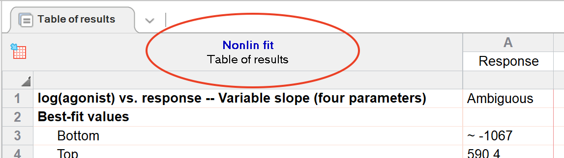
Note the word 'ambiguous' at the top of the results. This means that Prism was unable to find a unique fit to these data. Lots of sets of parameter values would lead to curves that fit just as well. Learn more about ambiguous fits.
Prism does not report confidence intervals for the logEC50 or the Bottom of the curve, but instead simply says the intervals are 'very wide'. That tells you it was impossible to fit those parameters precisely.
While the Y values of the data rum about 100 to about 600, the best-fit value for the bottom of the curve is -1067. Furthermore, the best-fit value of the logEC50 is outside the range of the data.
Even though the curve is close to the points (the R2 is 0.9669), the best-fit parameter values are useless.
9. Constrain the Bottom of the curve
The problem is simple. You have asked Prism to find best-fit value for four parameters representing the bottom and top plateaus of the curve as well as the mid point and steepness. But the data simply don't define the bottom of the curve. In fact, Prism the best fit value of Bottom is very very far from the data.
These data were calculated so the basal nonspecific response was subtracted away. This means that you know that the response (Y) at very low concentrations of agonist (very low values of X) has to be zero. Prism needs to know this to fit the data sensibly.
You don't have to do the fit over again. Instead click the button in the upper left corner of the results table to return to the nonlinear regression dialog.
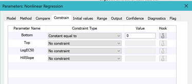
Go to the Constrain tab, and check constrain the parameter Bottom to have a constant value which you set to 0.0.
10. Inspect the revised results
Now the results make sense. The logEC50 is in the middle of the range of X values. The confidence intervals are reasonably tight. And, of course, the results are no longer 'ambiguous'.