1. Create a data table
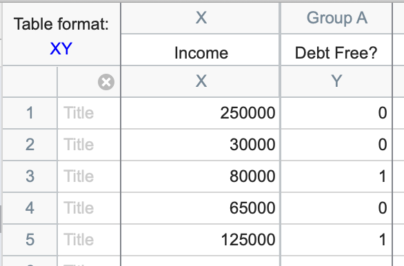
From the Welcome or New Table dialog, choose to create an XY data table. Be sure to select the option “Enter and plot a single Y value for each point.” Simple logistic regression in Prism currently does not allow for replicates in subcolumns. To enter replicates, simply add each replicate on its own row with its associated X value and observed outcome.
If you would like to see how Prism works on a sample data set, choose the sample data: Simple logistic regression. Otherwise, if you want to enter your own data, be sure that the Y values are binary and encoded as strictly 0s and 1s. Prism will not perform simple logistic regression (or multiple logistic regression) if your outcome variable is not encoded as 0s and 1s (read more about binary outcome variables).
Tip: An easy way to keep track of which outcome is coded as a 1 and which is coded as a 0 is to use a yes/no question as the title of your Y column. Using this method, you could enter a “1” to answer the question “yes” and a “0” to answer the question “no.”
2. Analysis choices
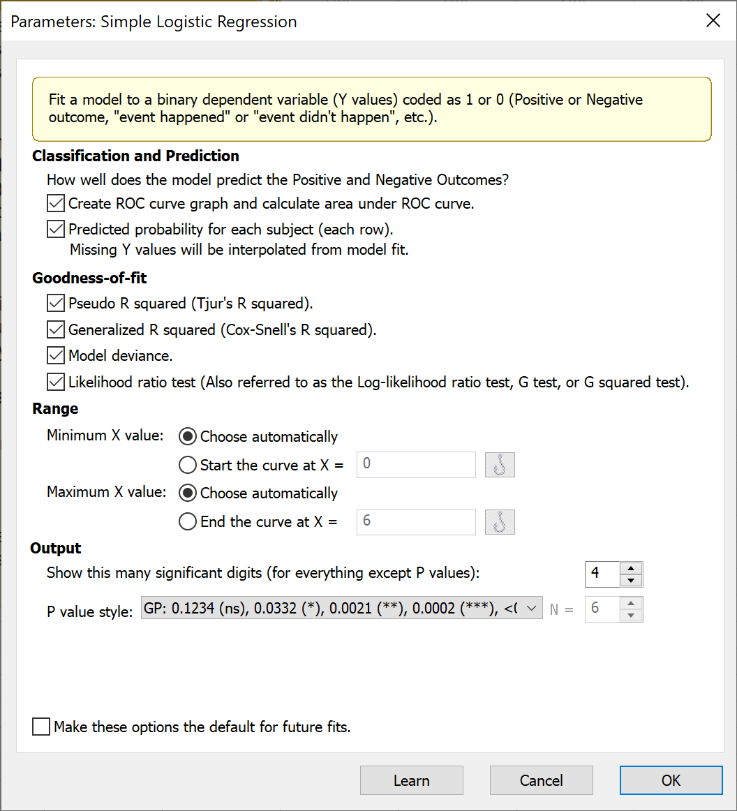
To run simple logistic regression, click the Analyze button in the toolbar and choose simple logistic regression from the list of XY analyses. The parameters dialog for simple logistic regression offers several customization choices. For even more analysis options, consider copying your data to a multiple variables data table and using the multiple logistic regression analysis.
a. Classification and interpolation
The options in this section provide information on how well the model does at predicting the positive and negative outcomes (entered as 1s and 0s in the data, respectively). You can request that Prism generate an ROC curve and report the area under the ROC curve (AUC) in the table of results. The AUC provides information on how well the logistic regression model classifies the observed data at various possible cutoffs. Check out this page for more on understanding ROC curves.
Selecting the “Classification of each subject” will output a new green table titled “Row Classification” that first copies the column of observed X values and adds a column containing the predicted probabilities for each of those values from the simple logistic regression model. Note that you can use this option to predict new observations at specific values of X. To do this, simply add a row at the bottom of the original data table with the desired X value (or values) and leave the corresponding Y values blank (note that this process is very similar to the way interpolation is performed for simple linear regression, but is done automatically without selecting additional options).
b. Goodness-of-fit
In addition to classification performance, Prism offers four ways to evaluate model performance.
The standard metric for evaluating the fit of a linear model is R squared. However, because the simple logistic regression model is not fit using the same techniques as simple linear regression, this metric is not appropriate for logistic regression. For simple logistic regression, Prism offers two alternatives to R squared. Although these have the term R squared in their name, they do not have the same interpretation as R squared from simple linear regression (i.e. they do not represent the proportion of variance explained by the model).
Instead, both Tjur’s Pseudo R squared and Cox-Snell’s Generalized R squared are values that range between 0 and 1, with larger values representing better predictive performance of the model. More details on these pseudo R squared metrics (and others offered through multiple logistic regression from the multiple variables data table) can be found here.
Model deviance produces a value sometimes referred to as G squared which is used to calculate the test statistic for the likelihood ratio test. If you are comparing different X predictors for your model, you can choose the predictor that results in the smallest model deviance. You can also use the Pseudo and Generalized R squared values in this way.
The likelihood ratio test (LRT) compares the logistic model that includes the given X predictor to a model without that X predictor (i.e. an “intercept-only” model). Like other hypothesis tests, the LRT uses a null hypothesis, and generates a P value to test that null hypothesis. In this case, the null hypothesis is that the intercept-only model (the model without the X variable) fits the data better than the model with the X variable. If your X variable contributes to model prediction performance, you would expect that the P value for this test would be small.
c. Range
A logistic plot is automatically generated when you perform simple logistic regression. You can allow Prism to choose the default minimum and maximum X values for plotting this curve based on your data, or you may choose to increase or decrease these limits as you choose.