While fitting a nonlinear regression model, you may also be interested in various transformations, combinations, and interpolations of the best-fit parameter values. Using the "Transforms to Report" tab of the model definition dialog, these values can be defined for Prism to report (along with their confidence intervals when applicable) on the reported results.
Defining parameter transformations
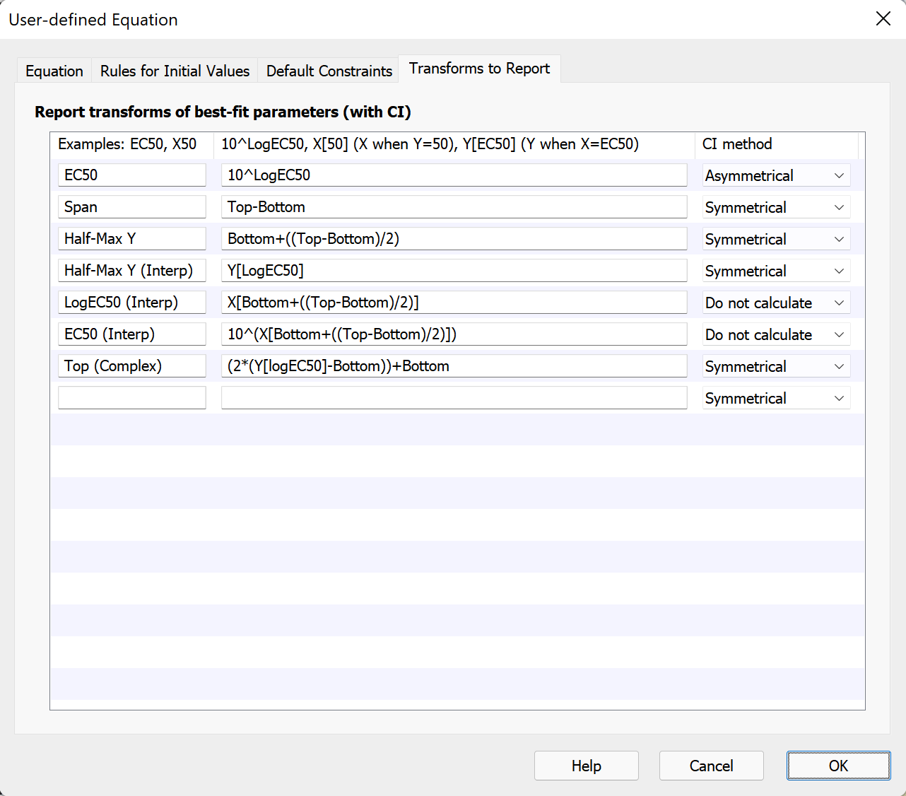
Give the transformation a name
The far left text box on each row of the Transforms to Report dialog is used to name the transformation for that row. This is the name that will be displayed in the table of results for the nonlinear regression, so choose something that you’ll recognize.
Define the transformation or interpolation
The second text box on each row of the dialog is for the definition (equation) that will be used to calculate the desired transformation or interpolation. Note that you can use any combination of model parameters when defining the transformation. However, you cannot use the result of one transformation as the input for another. The inputs to the transform can only be parameters fit by the regression or standard mathematical operators (log, exp, etc.). Because these definitions are for transformations of parameters, it would make no sense to include X or Y in the transform (although interpolations can be used).
Example: you fit data to an equation that includes the parameter “logEC50” that is the logarithm of an EC50, but you also want to include a value and error estimate for the EC50 based on the best-fit model parameter values. Enter the label “EC50” in the left text box and enter “10^logEC50” in the right text box (without the quotes).
Example: You fit data to an equation that reports a rate constant “K”, but you would also like to report the half-life. Enter the label “Half Life” in the left text box and enter the definition “ln(2)/K” in the right text box (without the quotes).
You can also use the “Transforms” controls to report values calculated from the curve of best-fit parameter values. The interpolated value and its confidence interval (if applicable) will appear in the results along with other transformed parameters. If an interpolation is included in the definition, the interpolation can be based on a constant value (a number), a single parameter, or a combination (function) of multiple parameters. Use the following syntax:
•Y[constant value or parameter]
The Y value of the curve when X is the value entered within the brackets. The Y value will be computed for any X, but confidence intervals will be calculated only when the X value is within the range of the X axis
•X[constant value or parameter]
The X value of the curve when Y is the value you enter within the brackets. Prism searches for the Y value entered within the range that the curve is plotted (Range tab) extending in both directions a distance equal to half that range. It reports the smallest X value it finds within that range that corresponds to the Y value entered, and doesn’t alert you when the curve oscillates so that there are several X values that correspond to a single Y value. If both X and Y are within the axis range, a confidence interval (if applicable) is also reported
Example: You've fit an inhibition dose-response curve, and you want to know the value of X when Y takes on a value of 50, even though this may not be the midpoint between the top and bottom plateaus of the curve (read more about relative and absolute IC50 here). For this, the interpolation definition would be:
•Absolute IC50 = X[50]
Advanced example: You want to calculate the value of Y that is halfway between the “bottom” and “top” plateau of a dose-response curve. There are two ways this could be done. The first is by using a transformation of the “Bottom” and “Top” parameters:
•Half-Max Y = Bottom+((Top-Bottom)/2)
An alternative method could be to use the LogEC50 parameter and an interpolation transform. Since LogEC50 is defined as the value of X (on the log scale) when Y is at half-maximum, the following interpolation would allow you to calculate Y at half-maximum from LogEC50:
•Half-Max Y (Interpolated) = Y[LogEC50]
The section “Types of transformations” below provides additional examples for each of the different possible transformations that can be performed in Prism.
Choose the confidence interval type
On each row, there is a dropdown menu that allows you to specify the type of confidence interval you would like to have reported for the defined transform. These choices are:
•Symmetrical
•Asymmetrical
•Do not calculate
The choice here can be a bit complicated since the options available for each row will depend on the transformation definition for that row, and the calculated results will also depend on the choice on the Confidence tab of the nonlinear regression parameters dialog for how the confidence intervals of the model parameters should be reported.
Because Prism allows transformations that include any combination of model parameters and interpolations, the specific options available in this dropdown menu will depend on the type of transformation defined (see the section “Types of transformations” below for more information).
Our recommendation: Choose “Asymmetrical” if this choice is available; otherwise choose “symmetrical”. Also, in the Confidence tab of the nonlinear regression dialog, we recommend always choosing asymmetrical (profile likelihood) confidence intervals.
The rest of this page presents the different types of transformation available within Prism and the options available for each of them
Don't mix up confidence intervals of transformed parameters with confidence intervals of interpolated values
In spite of the fact that confidence intervals of transformed parameters and confidence intervals of interpolated values look the same in Prism’s results tables, they are actually quite different. The transform of a parameter could have been a parameter in the model had the equation been written differently. In contrast, an interpolation transform represents the predicted value of the curve at a specified point. The idea of a confidence interval from an interpolation transform is the same as the idea of the confidence band for the curve.
Note a potential point of confusion. Confidence intervals for interpolation transforms are reported in the same section of the results as simple transformations of model parameters. The title of this section depends on the confidence interval method selected on the Confidence tab of the nonlinear regression parameters dialog: either asymmetrical (profile-likelihood) CIs or as symmetrical (asymptotic, Wald) CIs. However, confidence intervals of interpolation transforms are calculated using a method that has to do with confidence bands, and has nothing to do with the method used to compute the confidence of the parameters (even though it is in a section labeled that way).
Note also that the concept of profile-likelihood confidence intervals cannot be applied to transformations of multiple parameters. Indeed, if this option is selected, no confidence intervals for transformations of multiple parameters will be reported.
Most of the time, Prism will automatically provide the most reasonable confidence interval (if it can be calculated), and the confidence interval options can be ignored. The option may seem simple enough, but there are a lot of mathematics behind these controls. Only read on if you are very interested in the specifics of how these CIs are calculated. With this information in mind, a summary of the different options available for each type of transformation can be found in the section “Types of transformations” below.
Types of Transformations
For the details of any particular type of transformation, find the appropriate section below. This chart provides a quick overview of the detailed information found below:
|
Confidence Interval Method (from Confidence Tab of Nonlinear regression parameters dialog) |
||||
Symmetrical (asymptotic) approximate CI |
Asymmetrical (profile-likelihood) CI |
||||
Confidence Interval Method (From Transforms to report tab) |
Confidence Interval Method (From Transforms to report tab) |
||||
Symmetrical |
Asymmetrical |
Symmetrical |
Asymmetrical |
||
No interpolation |
Transform of a single parameter |
Symmetric asymptotic CI |
Transformed asymptotic CI |
Transformed profile-likelihood CI |
Transformed profile-likelihood CI |
Transformation of multiple parameters |
Symmetric asymptotic CI |
Not applicable (cannot be selected in dialog) |
No CI reported (no accurate CI calculation available) |
Not applicable (cannot be selected in dialog) |
|
Y from X Interpolation |
Simple Interpolation, no additional parameters |
Symmetric asymptotic CI |
Transformed asymptotic CI |
Symmetric asymptotic CI |
Transformed asymptotic CI |
Complex interpolation, no additional parameters |
Symmetric asymptotic CI |
Transformed asymptotic CI |
Symmetric asymptotic CI |
Transformed asymptotic CI |
|
Interpolation with additional parameters |
Symmetric asymptotic CI |
Not applicable (cannot be selected in dialog) |
Symmetric asymptotic CI |
Not applicable (cannot be selected in dialog) |
|
X from Y Interpolation |
Simple interpolation, no additional parameters |
Not applicable (cannot be selected in dialog) |
Transformed asymptotic CI |
Not applicable (cannot be selected in dialog) |
Transformed asymptotic CI |
Complex interpolation, no additional parameters |
Not applicable (cannot be selected in dialog) |
Not applicable (cannot be selected in dialog) |
Not applicable (cannot be selected in dialog) |
Not applicable (cannot be selected in dialog) |
|
Interpolation with additional parameters |
Not applicable (cannot be selected in dialog) |
Not applicable (cannot be selected in dialog) |
Not applicable (cannot be selected in dialog) |
Not applicable (cannot be selected in dialog) |
|
Transformation of a single parameter, no interpolation
Transformation of multiple parameters, no interpolation
Transformation with simple Y from X interpolation, no additional parameters
Transformation with complex Y from X interpolation, no additional parameters
Transformation with Y from X interpolation and additional parameters
Transformation with simple X from Y interpolation, no additional parameters
Transformation with complex X from Y interpolation, no additional parameters
Transformation with X from Y interpolation and additional parameters
Additional notes about parameter transformations
•Prism 9.3 improved this feature. With earlier versions, you could only choose from a limited set of mathematical operators (sum, quotient, etc.) to combine two parameters. Starting with Prism 9.3, you can enter any equation you would like, and combine any number of parameters
•Prism 4 (and earlier) always reported asymmetrical confidence intervals for EC50 and half-lives, but did not offer the choice of transforming these parameters in user-defined equations
•When a transform simply changes units, symmetrical and “asymmetrical” confidence intervals are the same, so the choice doesn't matter. This is the case whenever the transform of a parameter “K” is of the form “a*K+b”
•Don't mix up the two choices for reporting the CI of transformed parameters discussed on this page with the two methods for reporting the CI of model parameters specified on the Confidence tab of the nonlinear regression analysis parameters dialog
•Prism only calculates confidence intervals for monotonic transformations. Otherwise, the results will be blank. What does it mean for a function to be monotonic? "A monotonic function is a function which is either entirely nonincreasing or nondecreasing. A function is monotonic if its first derivative (which need not be continuous) does not change sign." (1)
•When Prism reports the difference or ratio (etc) of two parameters, with standard error and confidence interval, the calculations account for the covariance of the two parameters. See this document.
References
1.Stover, Christopher. "Monotonic Function." From MathWorld--A Wolfram Web Resource, created by Eric W. Weisstein. https://mathworld.wolfram.com/MonotonicFunction.html