The term “censored” seems to imply that you or the subject did something inappropriate. But that isn’t the case. Survival analysis involves measuring the elapsed amount of time that passes between some defined “start time” and some other defined “end point” for each observation (subject, individual, etc.) in the sample population. Quite often, there are observations in a survival analysis for which this elapsed amount of time is unknown. These observations are said to be censored, and the reasons this could occur are explained along with an example below to make it easier to understand.
Consider a hypothetical clinical trial that is scheduled to last for 6 months, and that will include 20 participants. The enrollment criteria for this trial are such that only 8 of the 20 participants were identified at the time the trial began. The other 12 participants were recruited over the course of the next four months. Each participant was then followed until one of three things happened:
1.The participant experienced the event of interest (in this case, the participant died)
2.The participant dropped out of the study
3.The study ended after 6 months, but the participant did not die in that time
The graph below shows a timeline for each of the original 8 participants in the study, along with an indication of whether or not they died (event) or were censored.
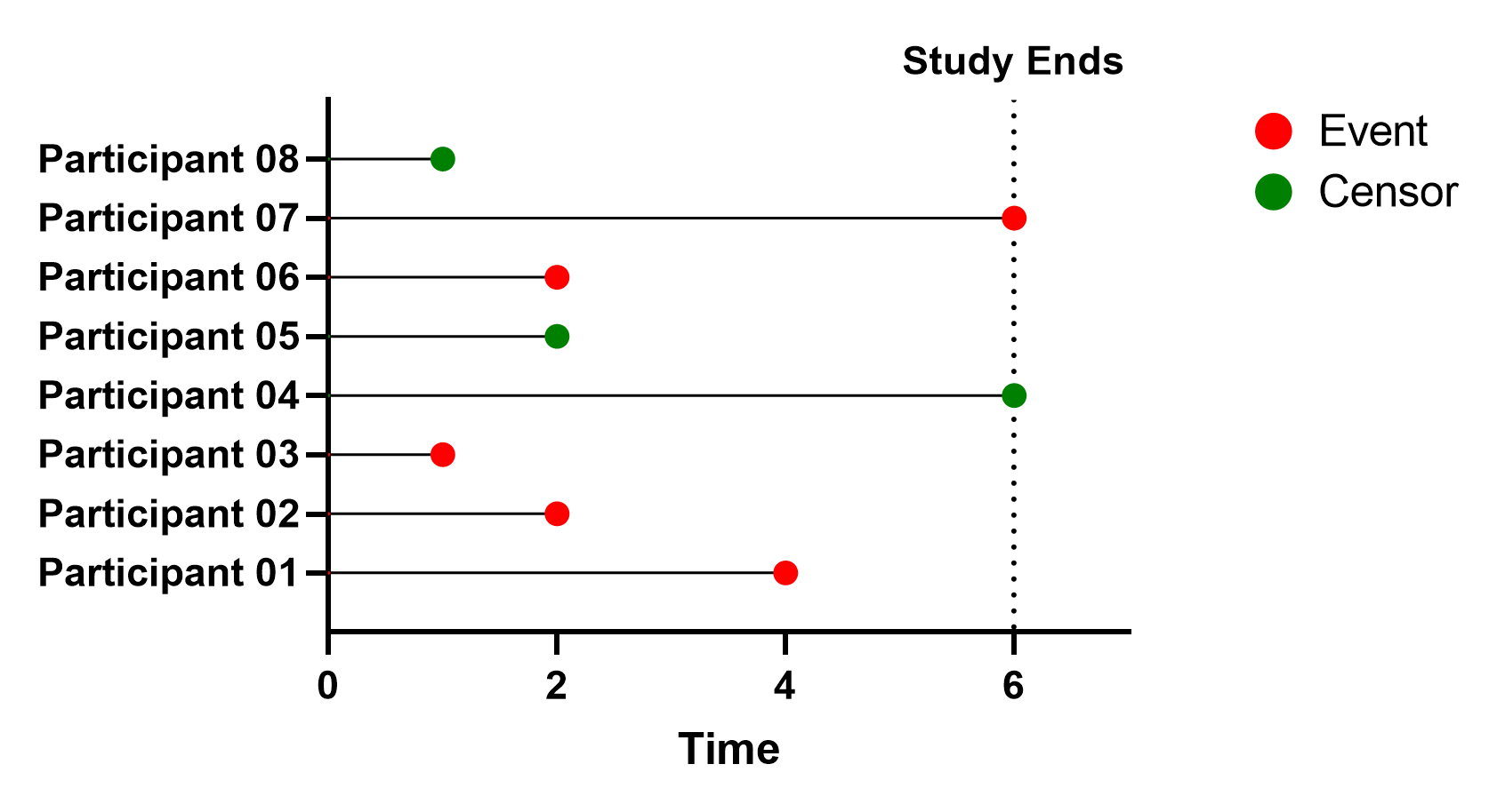
The graph above shows the “calendar time” on the X axis (the amount of time that has passed since the start of the experimental trial). Since the first eight participants entered the trial at the very beginning (time 0), the elapsed time to an event or censoring can be read directly from the graph. As shown in the graph above, Participant 01 was followed for four months, and then died. Similarly, Participants 02 and 03 were followed for two months and one month, respectively, and then each experienced the event of interest. Participant 07 was followed for 6 months, and died just before the end of the study. In contrast, Participant 04 was followed for the entire six months of the study, and did not experience the event of interest in that time period (they survived through the end of the study). Participant 05 was followed for two months, and did not die during this time. However, after these two months, Participant 05 chose to leave the study. Because Participant 05 was last seen at the two month mark, this is the time that we indicate that this individual was censored. Participant 08 was observed (and alive) at the one-month time point, but also left the study after just this one month. Note the difference between Participants 04 and 07. Although both participated in the study for six months, we know that Participant 07 died at the six month time point, while Participant 04 survived through the end of the study.
For Participants 04, 05, and 08, we can’t know how much time passed before they experienced the event of interest, only that it must occur after the last time that each of them was last observed. From these original eight participants, we can only state that five experienced the event of interest, while these other three were censored.
Now that we have an idea of what this visualization tells us, we can look at all of the other participants in the study to get a complete picture of the data.
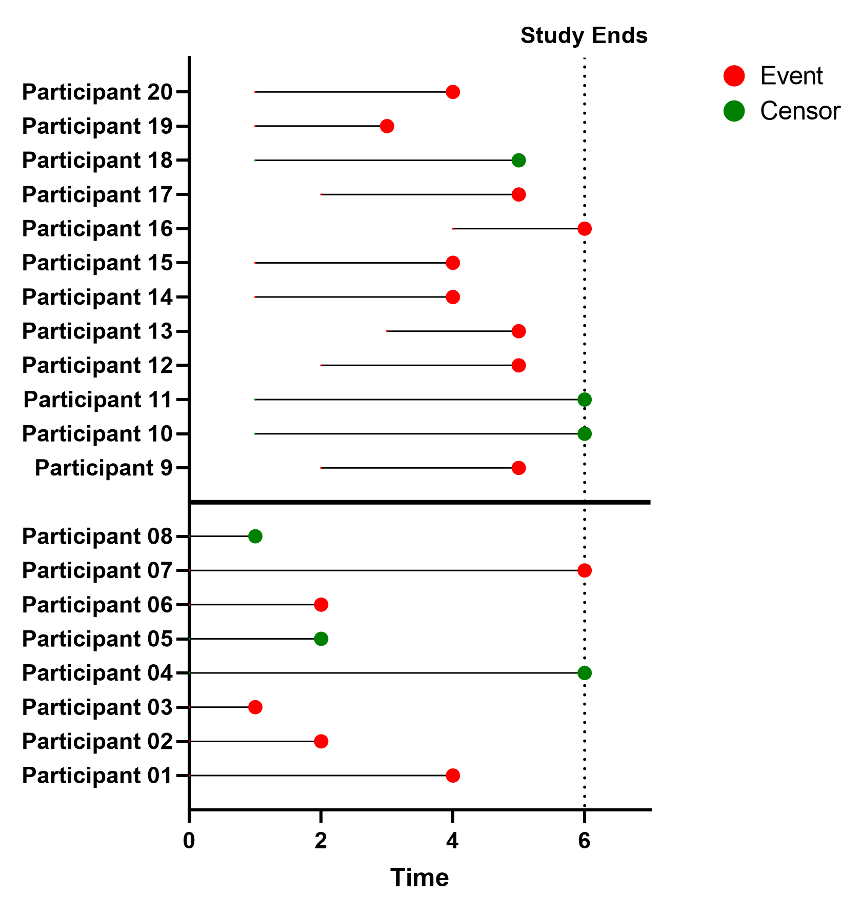
Twelve additional participants were recruited after the study began (Participants 09-20). As before, the graph above shows “calendar time” on the X axis. But we can see that the “start time” for participants 09-20 is no longer at Time = 0. Because the start time and end time for each participant may be different, we must find the difference between these two values to determine the “elapsed observation time” for each participant individually. Using the graph above, we see that seven of the next 12 participants were recruited after one month, three after two months, and one each after three months and four months respectively. Because of this, we cannot simply read off the event or censoring time as the elapsed time since these individuals did not start at time zero.
Of the twelve participants recruited after the beginning of the study, one (Participant 18) left the study and two did not experience the event of interest before the end of the study, resulting in three additional censored observations and nine additional observations for the event of interest.
This method of censoring is known as “right-censoring” since the survival time of the censored participant is unknown on the right hand side of the timeline. In other words, the event must have occurred after the observation period for each of these participants. There are other methods of censoring (with left-censoring and interval-censoring being the most common), however right-censoring is what will be used for survival analysis within Prism.
The following sections of this guide will cover information on the two types of survival analysis offered by Prism:
•Nonparametric survival analysis: Does not allow for multiple predictor variables or continuous predictor variables. Uses the Kaplan-Meier (product limit) method to estimate the survival function (survival curve). Separate curves for different groups (defined by a single categorical variable) can be compared using the logrank (Mantel-Haenszel, Mantel-Cox) and/or Gehan-Wilcoxon tests
•Semiparametric survival analysis: Uses Cox proportional hazards regression to estimate hazard ratios and parameter coefficients, baseline cumulative hazard and survival curves, and survival probability estimates for each observation. Allows for inclusion of multiple continuous and categorical predictor variables
A third type of survival analysis - parametric survival analysis - requires additional assumptions about the distribution of survival times in the sample population, and is not currently offered as an analysis within Prism.