The primary objective of clustering analyses is to group the input data together into clusters based on the similarity (or dissimilarity) of each point to other points in the data. This is a fairly broad simplification of the process, but illustrates the overall goal of clustering: group similar things together while creating separate groups for things that are similar to each other, but dissimilar to things in different groups.

One of the most common ways to measure the similarity or dissimilarity of observations in your data is to determine their distance from each other. Just as you can consider the distance between two objects sitting on your desk as a measure of how close they are to each other, the distance between two observations in your data can be a measure of their closeness or similarity. Two objects that are closer together (that have a smaller distance between them) would appear more similar, while objects that are farther apart (that have a greater distance between them) would appear more dissimilar.

Where this gets somewhat complicated is that there are multiple different ways to measure the distance between two objects in your data! The following sections describe the distance metrics available in Prism along with some explanations for each.

Euclidean distance

The distance method that most of us are most familiar with is the Euclidean distance. This is the “straight line” distance between two points, and is the shortest path connecting them. The formula to calculate this distance in two dimensions (X and Y) is:

 

In higher dimensions, this formula can be expanded by simply adding additional terms within the square root. For example, with three dimensions (X, Y, and Z), the formula is:

For points A = (a1, a2, a3, …) and B = (b1, b2, b3, ...). This distance metric is sometimes referred to as the “L2” distance as it involves raising the differences between values in the formula to the second power (squaring them) and taking the square root. This distance metric is available for both hierarchical clustering and K-means clustering, and is commonly used as a default distance metric.

Manhattan distance

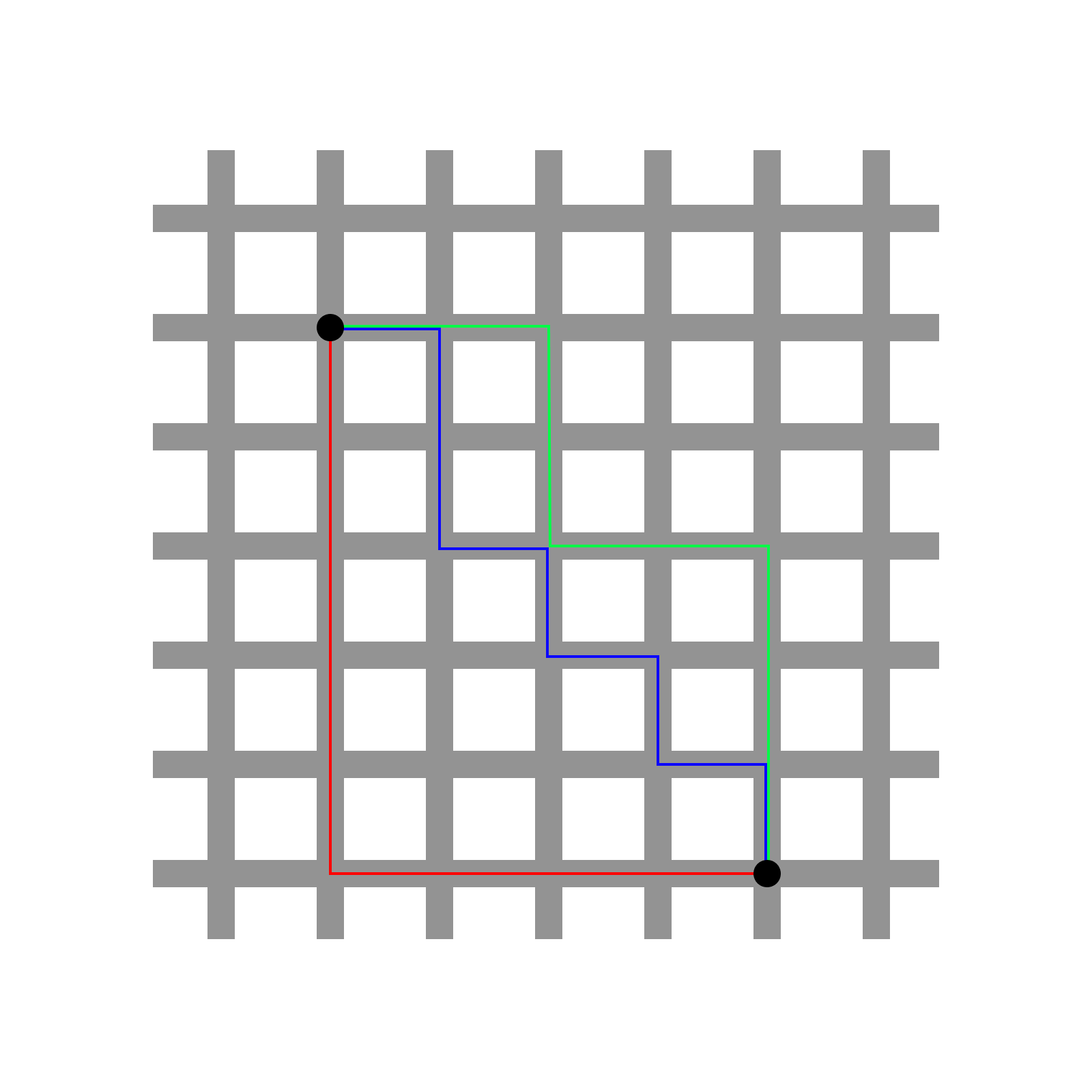
The Manhattan distance is sometimes referred to as the “taxicab” distance due to the manner that it’s most easily understood. Consider a grid pattern of roads that all intersect at 90 degree angles. If you wanted to take a taxi to get from one intersection to another, you could not travel diagonally “through” the city blocks, but rather travel in straight lines along the roads. The smallest number of blocks that you would have to travel to get from one intersection to another is the Manhattan (or taxicab) distance between these two points. In the image below, there are three possible paths (and many others) to get from one black point to another on the grid. However, the number of blocks traveled along each of these paths is the same (they all require traveling nine blocks). This value is the Manhattan distance between these points.

The formula for the manhattan distance for two variables (X and Y) is given as:

In higher dimensions, this can be generalized as:

For points a = (a1, a2, a3, …) and b = (b1, b2, b3, ...). This distance metric is sometimes also referred to as the “L1” distance, and is available for both K-means and hierarchical clustering in Prism.

Pearson correlation distance

To understand the Pearson correlation distance, it’s easier to consider the “points” being used to calculate the distance as variables. Consider two variables A (with values a1, a2, a3, …) and B (with values b1, b2, b3, …). The Pearson correlation coefficient between these two variables is a measure of their linear relationship, and is defined as:

This correlation coefficient can take on a value from -1 (perfectly negatively correlated) to 1 (perfectly correlated). When two variables are perfectly correlated, the values of one variable increase as the values of the other variable increase. Conversely, when variables are perfectly negatively correlated, the values of one variable decrease as the values of the other increase. Calculating the correlation distance from the correlation coefficient is simply a matter of subtracting the correlation coefficient from 1:

The motivation behind correlation distance is that in some cases it makes sense to consider two objects as being “close together” if their pattern of values (correlation) - but not the specific values within the variables - are similar. Because the Pearson correlation coefficient values can range from 1 (perfectly correlated) to zero (no correlation at all) to -1 (perfectly negatively correlated), it follows that the correlation distance can take on values from zero to 2. When two objects/variables to be clustered are perfectly correlated (r = 1), then their correlation distance is zero (d = 1 - 1 = 0). In other words, they’re as close as they can be! When these objects are perfectly negatively correlated (r = -1), their distance from each other is two (d = 1 - [-1] = 2), which is as far apart as two objects can be using this distance scale.

Finally, note that the Pearson correlation coefficient is not changed by scaling of the data, so if you’re clustering on columns using the correlation distance, it won’t matter if you choose to standardize or center the data within columns. The same applies for clustering and scaling on rows.

A slight modification of this approach is sometimes called the “absolute correlation distance”, and considers the absolute value of the correlation coefficient in the distance calculation:

Here, two variables are considered to have a distance of zero if they are perfectly correlated OR if they are perfectly negatively correlated. This method of distance calculation may be interesting for certain gene expression studies where it would be considered no more interesting for two genes to follow the same exact pattern of expression than for them to follow a perfectly inverted pattern. The absolute correlation distance is not yet available in Prism, but will be added soon.

Cosine distance

To understand how the cosine distance is calculated, it’s useful to consider the objects to be clustered as vectors. Consider two vectors A (a1, a2, a3, …) and B (b1, b2, b3, …). The cosine similarity between these two vectors is the cosine of the angle formed between them, and is defined as:

As this value is calculated using the cosine function, it can take on values ranging from -1 to 1. When two vectors are perfectly aligned, the angle between them is zero, and the cosine of the angle is 1. When two vectors are orthogonal, the angle between them is a right angle (90°), and the cosine of this angle is zero. Finally, if two vectors point in perfectly opposite directions, the angle between them is 180° and the cosine of this angle is -1. Once the cosine similarity is calculated, it’s easy enough to determine the cosine distance, which is defined as:

The motivation for the cosine distance is that two vectors that point in the same direction should be considered to be very similar (they will have a cosine similarity close to 1), and so the “distance” between them should be nearly zero. You can see from this definition that when cosine similarity is 1, the cosine distance is zero. When two vectors are perpendicular (orthogonal), the cosine similarity is zero, and the cosine distance of these vectors is 1. Finally, when two vectors point in opposite directions, their cosine similarity is -1, so their cosine distance is 2 (as far apart as possible on this scale).