When performing any type of regression, it is often of interest to investigate how well the model describes the data compared to other possible models that could be fit. Prism provides a number of methods that can be employed to provide information on this idea of how well the model fits the provided data. Specifically, for Cox proportional hazards regression, Prism will report values for Akaike’s Information Criterion (AIC), the partial log-likelihood (LL), a transform of the partial log-likelihood (-2*LL), and pseudo R squared.
Akaike's Information Criterion (AIC)
This value is derived from an information theory approach that attempts to determine how well the data fit the model. The reported value depends both on the partial log-likelihood (described below) as well as the number of parameters in the model. Note that because it is difficult to specify the number of observations in the presence of censoring, Prism - like other applications - only reports AIC, and not corrected AIC (AICc). The equation needed to calculate AIC is given below:

where k is the number of parameters in the model (reported by Prism in the data summary section of the results).
Interpreting AIC
The interpretation of AIC relies heavily on the concept of the likelihood (more specifically, the log-likelihood or - in the case of Cox regression - the partial log-likelihood) of the model fit. Without going too far into the mathematics behind likelihood, the general idea is that the likelihood of a model tells you how how well the data fit that model (another way to think about it is how "likely" it is that these data were generated if you assume that the selected model is the "true" model). With this in mind, it should make sense that "good" models result in a higher value of likelihood while "poor" models have a lower value for their likelihood.
In the equation above, we see that AIC depends on two things:
1.The partial log-likelihood of the model
2.The number of parameters in the model (k)
The partial log-likelihood for a Cox regression model is simply the logarithm of the partial likelihood. As mentioned above, models which the data fit well will have higher likelihoods than models which the data do not fit well. Thus, the partial log-likelihoods for models which the data fit well will also be larger than the partial log-likelihood for models which the data fit less well. By multiplying this value by a negative value, we can see that models which the data fit better will result in a smaller value for "-2*(partial log-likelihood)" than models which the data fit less well. Thus, we can see that a larger likelihood ultimately results in a smaller AIC (ignoring the 2k term which will be discussed shortly). So it makes sense that a smaller AIC represents a "better" model fit.
The second part of the AIC equation is a "penalty" term that tries to prevent over-fitting (using too many parameters in a model). For any model, adding additional parameters (without changing anything else) will generally always increase the likelihood of the resulting model fit. With enough parameters, you will be able to perfectly predict the data in your input dataset (but this model will almost certainly do a terrible job predicting values for future observations outside of the input data). This is the problem of over-fitting: the model fits to the input data too well. The AIC formula adds a value equal to twice the number of parameters in the model (2k), so that models with more parameters have more of a "penalty" added to their AIC value.
Using all of this information, we can start to understand AIC a bit more:
•A model with a small AIC value suggests a better fit than a model with a large AIC value on the same data
•Models with more parameters will have larger likelihood values, but will also have a larger "penalty" added to their AIC value
The last very important concept to note about AIC values is that they can only be compared between models fit to the same data! AIC values are calculated from likelihood, which is specific to the data set being analyzed. Thus, it doesn't make any sense to try and compare AIC values for models fit to different data sets. Note also that it is the difference of AIC that we use to assess if a model fit is "better" or worse than another, not the ratio of AIC values. This ratio can not be directly interpreted, and so is not reported.
So then the best way to interpret AIC as reported in Prism for Cox regression is to compare the AIC value provided for the specified model against either the null model of another (competing) specified model fit to the same data. When comparing to the null model, a smaller AIC for the specified model suggests that the selected parameters improve the fit of the model. When comparing two competing models, the model with the AIC is considered to be a better overall fit while accounting for the number of parameters included in each model.
Advanced information on AIC
When comparing models (for example, comparing two competing models on the same data or comparing a specified model with the null model) it's possible to use the corresponding AIC values for each model to calculate a "probability" that each model is correct (under the assumption that these are the only possible models, and thus one of them must be correct). To do this, we can use the difference between two AIC values. First, let's define a new value for each model:

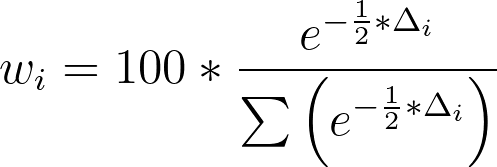
where AICi is the AIC of the individual model and min(AIC) is the smallest of all possible AIC values from the models being compared. Note that for the model with the smallest AIC value, AICi will be the same as min(AIC), and so Δi for this model will be zero. Once we have these values of Δ for each model, the "probability" that each model is correct can be calculated using the following formula:
As an example, consider the comparison of two models with the following AIC values:
•Model 1 AIC: 283
•Model 2 AIC: 285
The Δ values for these models is thus:
•Model 1 Δ: 0
•Model 2 Δ: 2
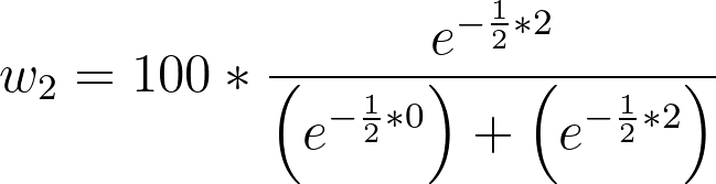
And the probability that each model is correct is calculated as:
•Model 1 w: 73.11%

•Model 2 w: 26.89%
This method can be extended to account for the comparison of any number of models, but remember that the assumption with this approach is that one of the models being compared is the "true" model (though this assumption may not be at all true in practice).
Partial log-likelihood (LL)
The concept of likelihood is mathematically quite complex, and is used in the process of estimating the best-fit parameter values as part of Cox proportional hazards regression analysis. However, the way that the partial log likelihood can be used to assess the model fit is (fortunately) quite simple. In general, when comparing two models fit to the same data, the model with the larger log likelihood is considered a better “fit”. Note that these log likelihood values are often negative! In this case, the larger value is the same as the less negative value. Thus the model with the less negative value is considered the model with a better "fit".
When this option is selected, the partial log-likelihood value will be given in the results for a model with no covariates (the null model) and the specified model. If the partial log-likelihood for the selected model is smaller than the negative log likelihood for the null model, it means that the input data were more likely to be generated by the specified model than by the null model. However, the AIC values for each model are generally used to determine which is "better" (with the smaller AIC value representing a "better" model fit).
Negative two times partial log-likelihood (-2*LL)
Like the other values reported by Prism in this section of the results, this value is related to the partial log-likelihood, and can be used to assess how well a model fits to the given data. As discussed previously, this value of "-2*(partial log-likelihood)" is used directly when calculating AIC. Fortunately, once you’ve obtained the partial log-likelihood (reported by Prism), calculating this value is as simple as multiplying by -2! Other programs and books will sometimes report this formula in other equivalent ways:


Pseudo R2
When considering “goodness-of-fit” for regression analyses, the concept of R squared normally comes up. This metric provides an estimate for the variance explained by the model, and is very useful when performing multiple linear regression, but there is no way to calculate the same metric for Cox proportional hazards regression. As such, a number of other “pseudo R squared” analogues have been proposed. Note that these values do not have the same mathematical interpretation as R squared. Pseudo R squared values do not represent the proportion of variance explained by the specified model. Instead, these pseudo R squared values are typically used to compare the goodness of fit for multiple models on the same data.
If selected in the parameters dialog of Cox proportional hazards regression, Prism will report Cox-Snell’s R squared (sometimes referred to as the “generalized” R squared). This value is calculated using the likelihood values of both the specified model and the null model (model with no covariates) according to the following formula:
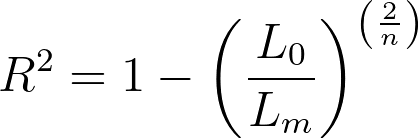
Where Lm is the partial likelihood (note, not the log-likelihood) of the specified model, L0 is the partial likelihood of the model with no covariates (the null model), and n is the number of observations used in the model (including censored observations).
From the equation for this pseudo-R2, we can see that when a model fits the data better (a higher partial likelihood value for Lm), the fraction becomes smaller, and the R2 value is larger. When the partial likelihood for the given model is smaller, the fraction is larger, and the corresponding R2 value is smaller. Like the R2 value seen in normal (least squares) regression, this formula has a minimum value of 0 (if the partial likelihood of the specified model is the same as the null model, R2 will equal zero). However, unlike the standard R2, the upper limit of this pseudo-R2 is not 1! Instead, if the model fits the data perfectly and the likelihood of the model is 1, then the resulting equation is:
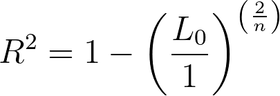
The partial likelihood of the null model is generally extremely small, but not zero. Thus, the maximum value for the Cox-Snell R2 depends on the likelihood of the null model, and may be very close to 1 (sometimes so close that computers can’t calculate the difference), but may not necessarily be equal to 1.
To summarize:
•The minimum value of this pseudo R2 is 0.0
•The maximum value of this pseudo R2 is less than 1.0, but in many cases very very close to 1.0