When performing regression, strongly correlated predictor variables (or, more generally, linearly dependent predictor variables) cause estimation instability. This often means that the estimates generated by the regression cannot be accurately interpreted. The reason for this is that - when two predictor variables are linearly dependent - one variable can be used to predict the value of the other. Another way to say this is that one variable can be written as a linear function of the other. For example, predictor variables X1 and X2 would be linearly dependent if the formula X2 = 3*X1 + 6 was true. For any given value of X1, a value of X2 would be known (and would, thus, not need to be estimated). If this were the case, the inclusion of X2 would add no new information to the model that couldn’t already be described by X1.
In multiple regression analysis, this problem is known as multicollinearity. In extreme cases, when one predictor variable is perfectly linearly dependent with another, the optimization algorithms required for completion of the analysis cannot determine the coefficient estimates for either column. This is because there would be an infinite number of potential solutions for these parameter estimates. An example to make this concept clear might involve a dataset in which two variables were both included with values of weight, one recorded in pounds and one in kilograms. Since these values are perfectly linearly correlated (pounds = 2.205*kilograms), a model that included them both would be unable to determine parameter estimates for either of them.
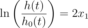
Consider the following case for Cox proportional hazards regression. Let’s assume there is only one predictor variable (x1) and the best-fit parameter estimate for this predictor variable is two. The Cox regression model would be:
Now, let’s assume we add a new variable (x2) that is a copy of the first predictor variable. Knowing that x1 = x2, it can be seen that all of the following equations are equivalent to the first:
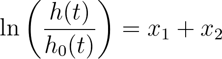
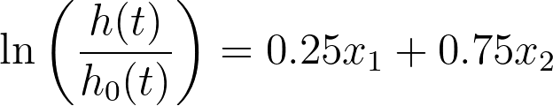
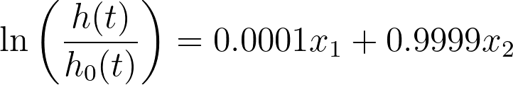
In fact, there are an infinite number of ways that this equation could be re-written with different coefficients, all resulting in the same values. In statistics, this model is said to be non-identifiable. In this extreme situation, standard errors, confidence intervals, and P values simply cannot be calculated.
However, it’s more common in practice that predictor variables aren’t perfectly linearly dependent with each other, but only strongly correlated. Although Prism will be able to generate parameter estimates in these situations, the problem still exists in that this multicollinearity increases uncertainty in the parameter estimates. This can be seen in the wider confidence intervals and larger P values.
If your only concern is using the model to predict future results from a defined set of predictor variable values, then large standard errors and wide confidence intervals might not be a major concern. However, if you are interested in the interpretation of the magnitude of a parameter estimate, then multicollinearity is a problem.
In Prism, multicollinearity is evaluated using variance inflation factors (VIFs). As a general rule of thumb, VIFs greater than 10 indicate strong multicollinearity and are likely detrimental to the model fit. In situations with VIFs of this magnitude, you’ll likely want to remove one of the predictor variables with a high VIF, and refit the model. This can be repeated as necessary. This page provides more detailed information on VIFs.