The objective of Cox proportional hazards regression is to build a mathematical relationship between the values of the predictor variables, and the hazard rate (hazard function) using the observed time-to-event data. From this information, it is possible to determine the survival function, giving us estimated survival for each individual as a function of time. However, for the sake of mathematical simplicity, the hazard rate is what is actually modeled. Here’s the general model that Cox proportional hazards regression is trying to define:

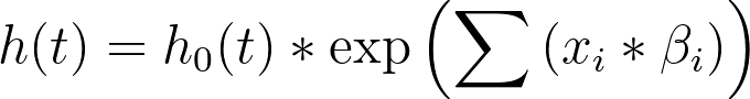
where:

•h(t) is the hazard rate (as a function of time)

•h0(t) is the baseline hazard rate (defined below)

•xi are the values of each predictor variable i - Note that elapsed time to the event of interest for each observation is not considered a predictor variable in Cox regression. Instead, the predictor variables represent any other measured variables that might have an effect on this elapsed (survival) time

•βi are the coefficients for each predictor variable i

One of the most important aspects of Cox proportional hazards regression is the assumption of the baseline hazard, shown as h0(t) in the equation above. This is itself a function of time that represents some curve (like the one shown in the previous section) that relates the frequency of the event of interest and time. Importantly, the specific shape of the baseline hazard is unimportant (it may start high and decrease over time; it may start low and increase over time; or it may contain many peaks and valleys throughout). In fact, performing Cox proportional hazards doesn’t require any knowledge of the shape or properties of the baseline hazard rate at all. This assumption that the baseline hazard can adopt any distribution is what makes Cox proportional hazards a semiparametric analysis.

The key point to know about the baseline hazard is that it represents the hazard rate when the values of all predictor variables have been set to zero (or their reference level for categorical variables). This can be shown using the equation above, setting xi to zero:

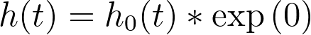
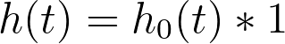
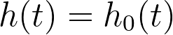
So the baseline hazard is the hazard function when the value of all predictor variables is set to zero! And the hazard for any individual in the population can be determined by multiplying this baseline hazard by some quantity determined by their specific values of the predictor variables (the part of the hazard rate equation above given by “exp(Σ(xi*βi))”). Another way to say this is that the hazard rate for any individual is proportional to a common baseline hazard rate.

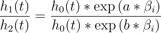
Another very interesting result of this assumption of a baseline hazard function is what happens when we consider the hazard for two individuals with different values of predictor variables. To keep it simple, let’s consider a model with a single predictor variable (xi), in which one individual has a value of “a” for this variable, and the second individual has a value of “b” for this variable. The hazard functions for these two individuals would be:

And the ratio of these hazard functions would be:

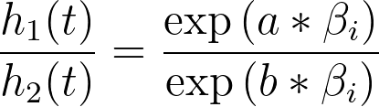
The baseline hazard in the numerator and denominator cancel, leaving a fraction that is constant with respect to time (we assume that the values of predictor variables don’t change over time). In other words, the hazard ratio for any two individuals in a population is constant at all times. Yet another way to say this, is that the hazards for two individuals in the population are always proportional to each other. This concept of proportionality is what gives this analysis its name: Cox proportional hazards regression. The following graph gives a graphical example of these proportional relationships: the black curve is a theoretical baseline hazard rate, while the blue and red curves represent hazard rates corresponding to two different values of a single predictor variable (some arbitrary value “α” for the blue curve, and double that value “2α” for the red curve):

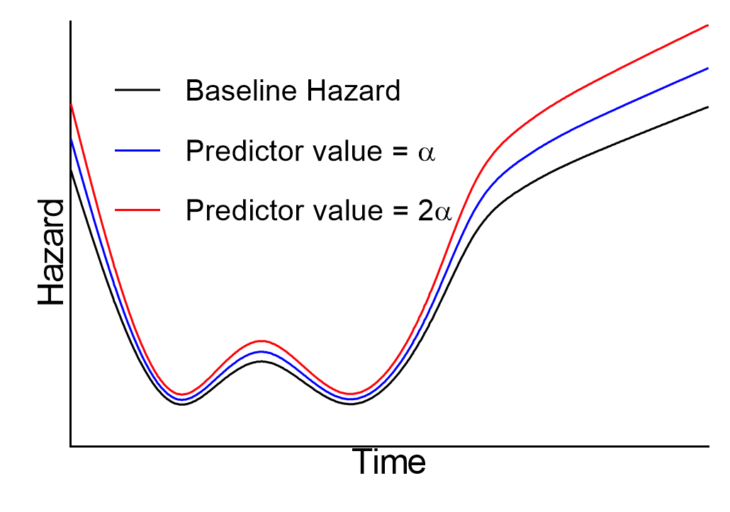
It can be seen that the vertical distance between each of these curves is not constant at all time points, but rather the ratio of the hazard for any two curves at any time will remain the same. Thus, as the value of the baseline hazard increases, the distance between the curves increases, while each curve retains a similar shape and - importantly - these curves never cross.

A later section will dig into the mathematical details of how these hazard rates are related to the survival function, which can be used to plot the estimated survival for any individual in the population at all times throughout the study given a set of values for the predictor variables in the model.