Let’s begin by defining the term hazard rate as the frequency at which the event of interest occurs per unit of time, given that it hasn’t yet happened up until that time. A higher hazard rate means more events occurring at a given time, while a lower hazard rate means fewer events occurring at a given time. Importantly, hazards can vary over time. Take the following graph for example:
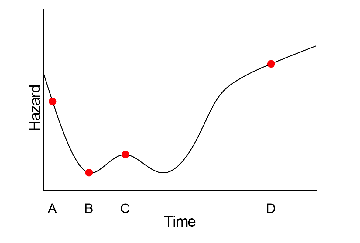
In this graph, the hazard starts somewhat high, then decreases for the first bit of time. It then increases to a small peak and decreases again, before finally increasing at different rates through the end of the observation period. The interpretation of this graph is that the risk of experiencing the event at time point A is higher than at B; the risk of experiencing the event at time C is lower than A, but higher than B; and the risk at D is higher than at A, B, or C.
While this graph is theoretical, it does have some similarities to actual hazard rates in human life expectancy. At birth, the hazard rate of death is actually much higher than shortly after birth. This hazard rate increases rapidly in the late teens to late twenties (with slight differences in men and women), and then continues to increase as time increases.
Something to be aware of is how hazards and time to event information are related. If the time to event data being observed is treated as discrete (i.e. events can only happen in a defined number of points in time), then the definition of hazard is relatively simple. The hazard, given by h(t) is defined as:
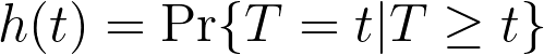
where “T” is a variable that represents the elapsed time at which the event could occur, and “t” represents a specific time of interest. The vertical line “|” is probability notation meaning “given that”. Thus, in words, the hazard rate is the probability that the event “T” occurs at time “t”, “given that” it has not happened prior to time “t”. However, when time is treated as continuous (as it almost always is in survival analysis), things get a little more complicated. Because time is treated as continuous, the event can happen in any given instant. There are an infinite number of possible “instants” in any defined window of time. Due to the nature of calculus, this means that the probability of the event happening at any one specific instant (T=t) is actually zero. Don’t worry too much about that if it doesn’t immediately make sense, just know that the mathematics required to calculate hazards when time is treated as a continuous variable (as it is in Cox proportional hazards regression), the calculations are a bit more complex.
In a later section, we’ll show (with a fair amount of math) that the hazard function and the survival function are directly related. However, without getting into the details, the important point to know is that it’s easier and more convenient to model the hazard function than to try and model the survival function directly. Thus, the objective of Cox proportional hazards regression is to estimate the hazard function. From this hazard function, the survival function (and estimates/predictions of survival) can be generated.