Overview
When you fit a curve with nonlinear regression, one of the most important set of results are the 95% confidence intervals of the parameters. These intervals are computed from the standard errors which are based on some mathematical simplifications. They are called "asymptotic" or "approximate" standard errors. They are calculated assuming that the equation is linear, but are applied to nonlinear equations. This simplification means that the intervals can be too optimistic, too narrow, so your true confidence level may be less than 95%.
How can you know whether the intervals really do have 95% confidence? There is no general way to answer this. But for any particular situation, you can get an answer using simulations. This page explains how to do this with Prism using the Monte Carlo feature new to Prism 6. We will simulate a dose-response curve and ask how accurate the 95% confidence intervals are for the Hill Slope. Christopolous suggested that the distribution of HillSlope can be asymmetrical, and suggested fitting the logarithm of the HillSlope instead (1).
Step 1. Simulating the first experiment
From anywhere, click New..Analysis and choose Simulate XY Data. To follow this example exactly, make these choices:
•X values tab. Start at X=-9, increment each X value by 0.5, and stop when X equals or exceeds -3.0.
•Equation tab. Choose the folder "Dose-response - Stimulation", and choose the equation: log(agonist) vs. response --Variable slope.
•Parameter values tab. Choose to simulate one data set, with 3 replicate values. Set Bottom=250, Top=5000, logEC50=-6, and HillSlope=0.5.
•Random error tab. Random error is Gaussian (absolute) with SD=200.
Step 2. Fit the first experiment
1.From the graph, click Analyze and choose Nonlinear regression. Or click the nonlinear regression shortcut button in the Analysis part of the toolbar.
2.On the first (Fit) tab, choose the folder: Dose-response - Stimulation. Then choose the equation: log(agonist) vs. response --Variable slope. You can accept all the defaults for the other tabs.
3.Click OK, and Prism will fit the model to the data and graph the curve on the graphs.
Step 3. Simulate a few more data sets
Note the Hill Slope, the parameter we wish to investigate in this simulation. To simulate new data with different random numbers, click the red die icon, or drop the Change menu and choose Simulate Again. Note that the Hill slope changes.
Step 4. Simulate many data sets
Start from the nonlinear regression results, click Analyze and choose Monte Carlo simulation.
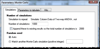
On the first (Simulations) tab, choose how many simulations you want Prism to perform. For this example, enter 1000.
On the second (Parameters to tabulate) tab, choose which parameters you want to tabulate. The choice is the list of analysis constants that Prism creates when it analyzes the data. For this example, we only want to tabulate the two confidence limits for the Hill Slope.
On the third (Hits) tab, define a criterion which makes a given simulated results a "hit". For this example, we'll define a hit to mean that the confidence interval brackets the true value of 0.5 (set in the simulation). So a hit is defined when the lower limit is less than or equal to 0.5 and the upper limit is greater than or equal to 0.5.
Click OK and Prism will run the simulations. Depending on the speed of your computer, it will take a few or a few dozen seconds.
Step 5. Monte-Carlo results
The results of the simulations are shown on only one page (since we unchecked all the options for reporting individual simulations in the Hits tab above.
The fraction of hits is 0954. For this example, we defined "hit" to mean that the confidence interval included the true parameter value. In other words, the confidence interval for HillSlope included the true value (used in the simulation) in 95.4% of the 1000 simulated data sets. (Since these results depend on which random numbers Prism generates, you'll get somewhat different results when you try to follow this example). This is what you'd expect for 95% confidence intervals, and means that you can trust the confidence intervals in experiment of this design. There is no need to consider fitting the logarithm of the Hill Slope instead, for this experimental design
Step 6. Try variations
If the confidence interval for this result is too wide for your tastes (it ranges from 93.9% to 96.6%), go back and run this Monte Carlo simulation with many more iterations (perhaps 10,000).
The conclusion is specific to the experimental design and parameter values you chose. Go back to the simulation, and change the HillSlope to 4.0. Then change the Monte Carlo dialog to redefine a "hit" to mean that the confidence interval brackets the true value of 4.0. A hit is defined when the lower limit is less than or equal to 4.0 and the upper limit is greater than or equal to 4.0. With such a steep HillSlope, the confidence intervals really are not accurate at all. The "95%" confidence intervals only include the true value (4.0) in 83.1% of the simulations. Doubling the number of concentrations (changing the increment of X values from 0.5 down to 0.25 in the X values tab of the Simulate XY data dialog) solves this problem. With so many data points, the 95% confidence intervals contain the true value in 95.3% of the simulations.
By varying the choices in the simulation dialog, and seeing the effect via Monte Carlo simulations, you can design better experiments.
Another example
Here is another detailed example, using simulations to find the power of a t test.
Reference
1. Arthur Christopoulos, Assessing the distribution of parameters in models of ligand-receptor interaction: to log or not to log, Trends in Pharmacological Sciences, Volume 19, Issue 9, 1 September 1998, Pages 351-357