To demonstrate how the calculations used in Kaplan-Meier survival analysis works, consider the following survival data:
Participant |
Time followed |
Event |
|---|---|---|
01 |
4 |
1 |
02 |
2 |
1 |
03 |
1 |
1 |
04 |
6 |
0 |
05 |
2 |
0 |
06 |
2 |
1 |
07 |
6 |
1 |
08 |
3 |
1 |
09 |
3 |
1 |
10 |
5 |
0 |
11 |
5 |
0 |
12 |
3 |
1 |
13 |
2 |
1 |
14 |
3 |
1 |
15 |
3 |
1 |
16 |
2 |
1 |
17 |
3 |
1 |
18 |
4 |
0 |
19 |
2 |
1 |
20 |
3 |
1 |
This data represents a study that included 20 participants, the elapsed amount of time that each participant was followed, and whether or not each participant experienced the event of interest or was censored (this is the same data used to generate the visualizations in the section discussing censoring).
The first step in manually generating a survival curve using the Kaplan-Meier method is to sort the data by elapsed time in ascending order (Prism does this “behind the scenes” for you so there’s no need to prepare your data this way when performing Kaplan-Meier analysis in Prism). The following table shows the re-arranged data:
Participant |
Time followed |
Event |
|---|---|---|
03 |
1 |
1 |
08 |
1 |
0 |
02 |
2 |
1 |
05 |
2 |
0 |
06 |
2 |
1 |
13 |
2 |
1 |
16 |
2 |
1 |
19 |
2 |
1 |
09 |
3 |
1 |
12 |
3 |
1 |
14 |
3 |
1 |
15 |
3 |
1 |
17 |
3 |
1 |
20 |
3 |
1 |
01 |
4 |
1 |
18 |
4 |
0 |
10 |
5 |
0 |
11 |
5 |
0 |
04 |
6 |
0 |
07 |
6 |
1 |
Now that the data have been arranged appropriately, the Kaplan-Meier approach can be used to estimate the survival probability at each time point at which an event occurs. To do this manually, we’ll need to identify a few pieces of information at each time point, including:
•The number at risk at time t (Nt)
•The number of events at time (Et)
•The number of censored observations at time t (Ct)
Before any time has elapsed for the individuals (time = 0), we have 20 total participants (all assumed to be “at risk”), and there are no deaths or censored observations at time zero. Therefore, the survival probability at time 0 is 1 (or 100%).
Elapsed time |
Number at risk (Nt) |
Number of events (Et) |
Number of censored (Ct) |
Survival probability |
0 |
20 |
0 |
0 |
1 |
Next, we add a row for each elapsed time that we have information about. It is important to note that an individual that experiences the event - or is censored - at time t is still considered to be at risk at time t. However, because we either know that they experienced the event or were censored, they are no longer included in the number at risk for any subsequent time points. Let’s start by adding one more row to the table:
Elapsed time |
Number at risk (Nt) |
Number of events (Et) |
Number of censored (Ct) |
Survival probability |
0 |
20 |
0 |
0 |
1 |
1 |
20 |
1 |
1 |
? |
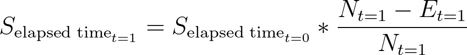
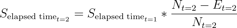
Looking at the original data, we see that at elapsed time = 1, there was one event (Participant 03) and one censored observation (Participant 08). Using this information, we can calculate the survival probability for this elapsed time using the following formula:
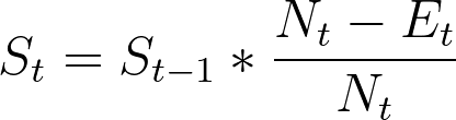
Using the numbers from the table above, we can calculate the survival probability as:
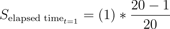
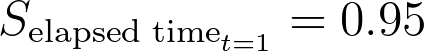
This means that there is an estimated survival probability (probability of not experiencing the event of interest) after one month of 95% in this population. Note that the number of censored observations (Ct) is not used in the calculation of survival probability (since we don’t know when these individuals actually experienced the event). However, it is used when calculating the number at risk for the next time point. It's probably clear why individuals that experience the event at a given time are not included in the "at risk" pool at later times (they already experienced the event). When an observation is censored at a given time, it means that this was the last time the individual was observed and that they had not yet experienced the event. However, because we can't know when this individual may experience the event, we cannot include them in the number at risk at later points in the study. Thus, the general formula for calculating the number at risk for a given time (Nt) is equal to the number at risk at the preceding time (Nt-1) minus the number of events and the number of censored observations at the preceding time. At elapsed time t = 1, we had Nt = 20, one event, and one observation. That means that at the next elapsed time point (t = 2), we’ll have 20 - 1 - 1 = 18 at risk. A new row has been added to the table for this next elapsed time point below:
Elapsed time |
Number at risk (Nt) |
Number of events (Et) |
Number of censored (Ct) |
Survival probability |
0 |
20 |
0 |
0 |
1 |
1 |
20 |
1 |
1 |
0.950 |
2 |
18 |
5 |
1 |
0.686 |
As before, survival probability was calculated as:
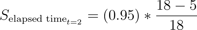
As before, this means that the estimated survival probability after two months is approximately 69% in this population. The rest of the table can be completed in a similar fashion:
Elapsed time |
Number at risk (Nt) |
Number of events (Et) |
Number of censored (Ct) |
Survival probability |
0 |
20 |
0 |
0 |
1 |
1 |
20 |
1 |
1 |
0.950 |
2 |
18 |
5 |
1 |
0.686 |
3 |
12 |
6 |
0 |
0.343 |
4 |
6 |
1 |
1 |
0.286 |
5 |
4 |
0 |
2 |
0.286 |
6 |
2 |
1 |
1 |
0.143 |
Using the values of Elapsed time and Survival probability from the table above, a stair-step survival curve can be plotted as shown below:
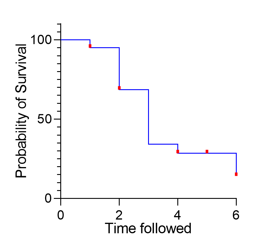
It was mentioned previously that censored observations aren’t used (directly) in the formula for calculating survival probability, but are used in determining the number at risk for the next time point. This can be seen in the table by looking at the calculated survival probability of elapsed times 4 and 5, and looking at the curve on the graph at Time followed = 5. On the graph, the red ticks indicate that an observation was censored at this time point, but because there is no vertical drop in the curve, it's apparent that no event occurred at this time point. Similarly, in the table, because the number of events (Et) was zero for time 5, the calculated survival probability did not change between this time point and the time point immediately preceding it.
Performing this sort of analysis within Prism is very simple, and Prism will automatically calculate and report all of these values along with the graph of the estimated survival probability. This section of the guide provides details on how to perform this analysis using Prism.