Principal component regression (PCR) is a combination of PCA and multiple linear regression (MLR). Often, the goal of dimensionality reduction via PCA is PCR, and Prism offers the ability to perform PCR as part of options in PCA. When choosing to perform PCR as part of PCA, the PCA results will include one additional tab of regression results in addition to the other results from PCA.
In brief, PCA is run, some number of principal components are selected, and MLR is run using those selected PC scores as independent (predictor) variables. Another variable, selected by you (and not included in the PCA) is the dependent (outcome) variable.
Prism does another step behind the scenes. Instead of reporting the regression coefficients on the scale of the PC scores, it transforms the regression coefficients back to the scale of the original input variables.
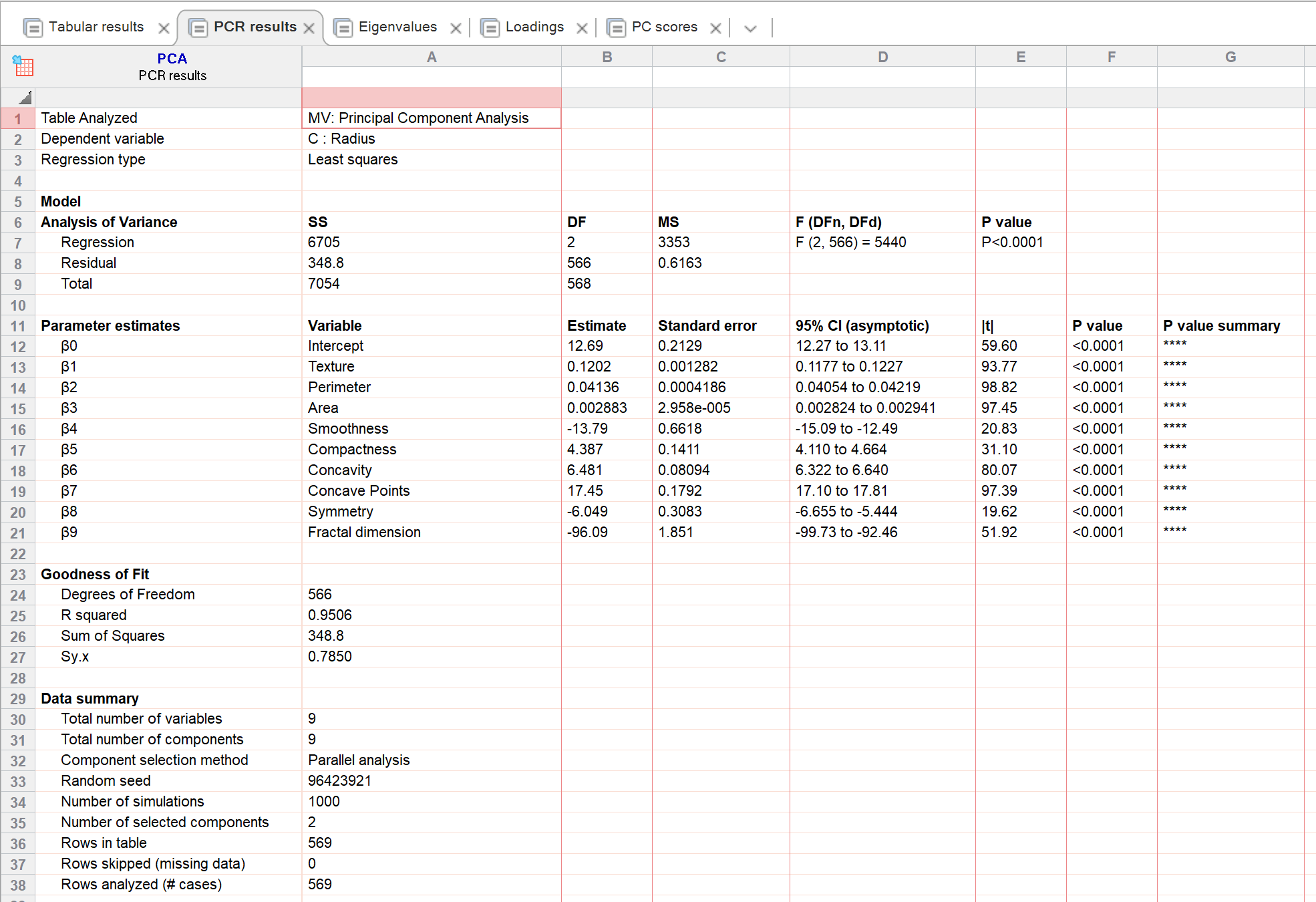
Notice that in the PCR results displayed below, the regression model used two degrees of freedom, because only two PCs were selected as independent variables. But note that coefficients are displayed for all nine independent variables plus the intercept. This seems mind-boggling, but is the whole point of PCR. Essentially MLR was fit on data that were projected into fewer dimensions (this probably sounds fancy, and is explained in greater detail here).
Other than fitting a MLR using the PC scores, the interpretation of the coefficients, standard error, and confidence intervals are the same as MLR. For example, the model is
estimated response = β0+β1*X1+β2*X2+β3*X3+ ...
Consult these additional pages for multiple linear regression to learn how to interpret the ANOVA table, P value, and R2.
Principal Components are the predictors of PCR, not the original variables
One quirk to note. Let’s start by calling the total number of data points (complete rows in the data table) “N”. Additionally, let’s call the number of chosen PCs (predictor variables) “k”.
The total degrees of freedom in the ANOVA table is defined as N-1. Why subtract 1? Because the intercept is fit. The degrees of freedom for the regression is defined to equal k, and the degrees of freedom of the residual is defined as N-k-1. A quick check shows that the degrees of freedom of the regression plus the degrees of freedom equals the degrees of freedom total:
dfreg + dfres = k + (N-k-1) = N - 1 = dftotal
In the Goodness of Fit section, degrees of freedom are defined as the total number of rows analyzed (N) minus the number of parameters. The number of parameters is different from the number of predictors since this model includes an intercept term. This means that the total number of parameters is equal to the number of predictors plus 1, or k+1. Thus, to calculated the degrees of freedom in the Goodness of Fit section, we end up with:
dfgof = N - (k+1) = N - k - 1
The example above has 569 rows of data, and the results table shows parameter estimates for 10 parameters (9 predictors plus the intercept). Yet there are only 2 degrees of freedom for the regression and 566 for the residual. That is because the regression actually only “saw” the two principal components as the predictors (or independent variables). As such, the degrees of freedom are computed as 569 - 3 = 566 (3, because it fit the two PCs plus the intercept). This is the “magic” of PCR. The PCA process reduces the number of independent variables down to a smaller number of principal components (without losing too much information), and so “gives” the analysis more degrees of freedom.
Data summary for PCR
Like the data summary for the Tabular results of PCA, the PCR results also include a Data summary section. Within this section, information is given pertaining to the number of original variables, PC selection method, number of selected components (used as the predictors for PCR), and rows of data in the data table. While these values will be the same for the Data summaries of both PCA and PCR, it is important to note that the final two rows with information on the number of Rows skipped (missing data) and Rows analyzed (# cases) may be different for PCR than for PCA.
Recall that in order to perform PCR, one variable from the input data table must be selected as the dependent (outcome) variable for the regression, and that this variable can not be included as a variable for PCA. Then, PCA is performed on the selected variables. If there are any missing (or excluded) values within these variables, those rows will be skipped during the PCA calculation. Afterward, PCR is performed using the calculated PCs and the indicated response (outcome, dependent) variable. For PCR, Prism checks if there are any missing (or excluded) values in the variables defining the PCs or in the response variable, and rows with missing values in any of these variables are skipped.
To make sure this point is extremely clear, here's another way to think about it. The components generated as part of PCA are defined using all possible data in the specified input variables (not counting the dependent variable). Those components are then used in regression with the specified dependent variable. If a row is missing a value for the dependent variable, that row is excluded from the regression, but other values on that row still play a part in determining the values of the principal components.
In summary:
•Rows skipped in PCA due to missing (or excluded) values will also be excluded in PCR on the same data
•Rows with missing (or excluded) values in a specified response variable will only be excluded in PCR. If a row is only missing a value for the response variable, but has values for all other input variables, this row will be used for PCA, but will be skipped for PCR
•As a result, it's possible to have a higher number for "Rows skipped (missing data)" from PCR than PCA for the same data