Two ways to analyze repeated measures data
Prism can analyze repeated measures data in two ways:
•Repeated measures ANOVA
•Fitting a mixed effects model. This analysis works fine even when there are some missing values. The results will only be meaningful, of course, if the values are missing for random reasons. For example, those results won't be helpful or meaningful if the values are missing because those participants were very sick, or those values were too high to measure (or too low to measure). Fitting a mixed model with missing values only makes sense when there is zero association between the treatments or time-points and the reason why some values are missing.
In general, fitting a mixed effects model is a much more versatile method. As implemented in Prism 8, the two are completely equivalent when there are no missing values. But the mixed effects model method can also fit data with missing values.
Analyze using which method
One-way, two-way, and three-way ANOVA offer the same choices for analyzing repeated measures data. They are on the Repeated Measures tab of the one-way and two-way ANOVA dialogs, and on the RM Analysis tab of the three-way ANOVA dialog. The screenshot below shows the one-way ANOVA dialog, but the choices on the relevant tab for each analysis are the same.
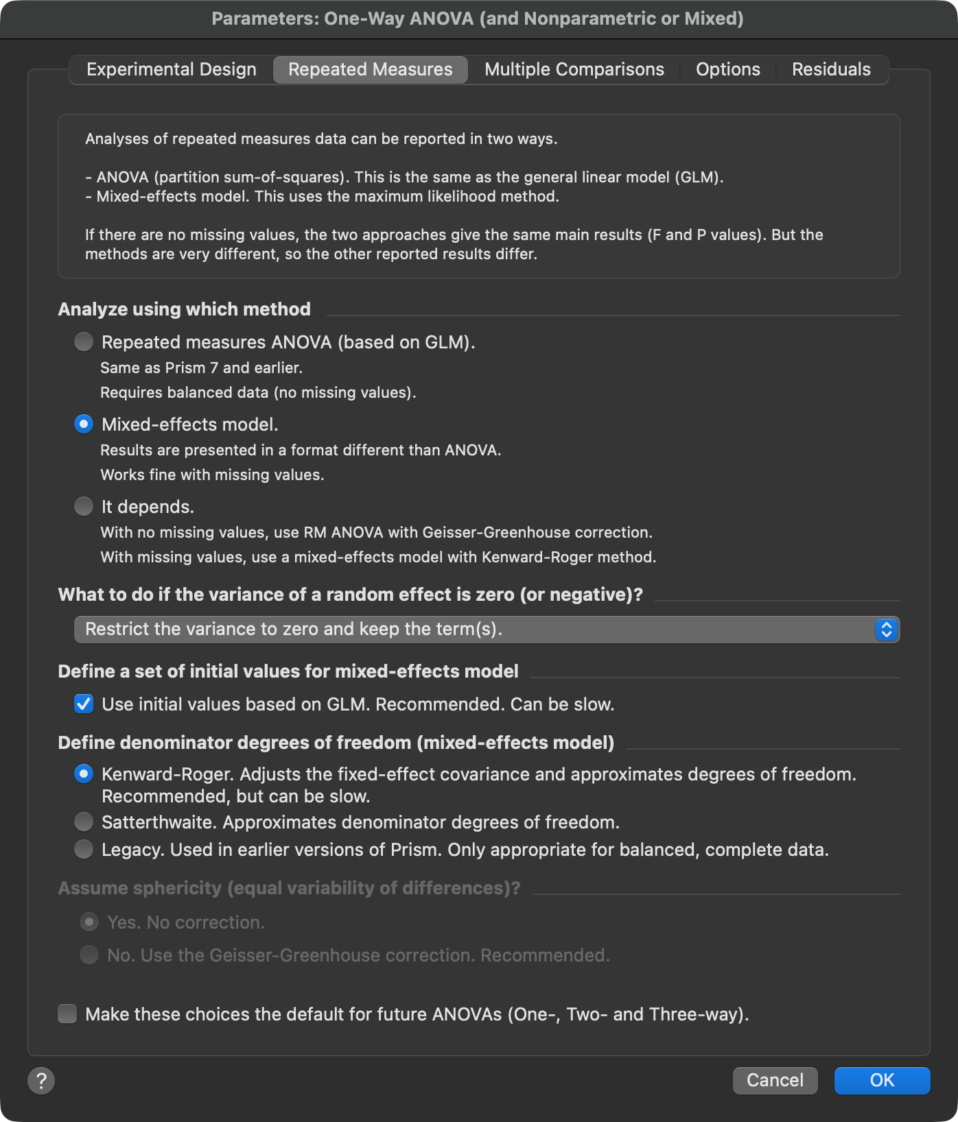
You have three choices for how to analyze the data:
•Use repeated measures ANOVA always. If there are missing values, no results will be reported. This matches what Prism 7 and earlier did. Prism is not "smart enough" to remove all data for a participant with missing values, but you could exclude all those values and rerun the ANOVA.
• Fit a mixed effects model always. This will make all analyses be consistent, whether or not there are missing values. If there are no missing values, the key results will be the same as repeated measures ANOVA but the results will be presented in an format unfamiliar to those used to repeated measures ANOVA.
•It depends. Report the fit to a mixed effects model only when there are missing values, when repeated measures ANOVA is impossible. When there are no missing values, report the familiar repeated measures ANOVA results, with the Geisser-Greenhouse correction. When there are missing values, Prism fits a mixed effects model and uses the Kenward-Roger method for the denominator degrees of freedom. This is the default.
Define denominator degrees of freedom (mixed-effects model)
When Prism fits a mixed effects model, the denominator degrees of freedom for each fixed effect test are not fixed by the design the way they are in ordinary ANOVA. This section gives you three ways to compute them:
•Legacy. Used in earlier Prism versions. Best for balanced, complete data. Not reliable when values are missing or the design is unbalanced.
•Satterthwaite. Approximates the denominator degrees of freedom from the uncertainty in the estimated variance components.
•Kenward-Roger. Adjusts the fixed-effect covariance and approximates the degrees of freedom. Recommended, and the default, but it can be slow on large models.
Your choice changes the degrees of freedom, the P values, and the confidence intervals, including those for multiple comparisons. It does not change the model fit, the estimated means, or the random effect SDs. For the full story, including how the Legacy method works and which option to pick, see denominator degrees of freedom in the mixed model.
This section is available only when you choose Mixed-effects model. It is unavailable when you choose repeated measures ANOVA, and when you choose It depends, because Prism then picks the method for you: Kenward-Roger whenever it fits a mixed effects model.
What to do if the variance of a random effect is zero (or negative)?
The whole point of repeated measures or mixed model analyses is that you have multiple response measurements on the same subject or when individuals are matched (twins or litters), so need to account for any correlation among multiple responses from the same subject. Mixed model analysis does this by estimating variances between subjects. In a simple mixed model, where only one variable is repeated, it’s possible that this correlation for the particular data in your study is zero or even negative (of course it is impossible for a variance to be negative, but it can happen with mixed effects models). Choose from the drop-down list what Prism should do when this happens:
•Restrict the variance to zero and keep the term(s). The term stays in the model with its variance held at zero, so the design you specified, including the matching, stays intact and your chosen degrees of freedom method stays available. This is the default.
•Remove the affected term(s) and fit a simpler model. Any random term whose variance is estimated to be zero or negative is removed, and Prism fits the simpler model. The removed term can be the subject term itself. If every random term is removed, the result is equivalent to ordinary ANOVA, and Prism posts a floating note saying so.
•Remove the affected term only if all interactions involving it are also affected. A zero-variance term is removed only when every interaction involving it is also estimated at zero. Otherwise its variance is restricted to zero and it stays in the model. Prism offers this choice only for models with two or more random effects, which means two-way or three-way ANOVA with repeated measures on more than one factor.
•Allow a negative variance estimate and fit the full model (matches SAS NOBOUND). No constraint is placed on the variance estimates. Analyses created in earlier versions of Prism that did not constrain the variance open with this choice.
Your choice here affects the degrees of freedom. Satterthwaite and Kenward-Roger degrees of freedom cannot be computed for a model with a term removed. If a term is removed, Prism falls back to the Legacy method for that result and posts a floating note saying so. If a variance is restricted to zero and the term is kept, Prism uses your chosen method, but those degrees of freedom are approximate, and a floating note tells you so.
Choose Restrict the variance to zero and keep the term(s) if you want to keep your chosen degrees of freedom method available.
In more complicated models, where there is more than one repeated measures variable, there are even more possible variance estimates (generally interactions with subject), and any of those could turn out to be zero or negative. The choice to remove a term only if all interactions involving it are also affected is designed for this case. It can remove a zero-variance interaction with subject, but it keeps the subject term in the model as long as any interaction involving subject still has a variance above zero.
Assume sphericity (equal variability of differences)?
Choose whether to assume sphericity. If you do not assume sphericity, Prism uses the Geisser-Greenhouse correction and reports epsilon.
This choice applies to repeated measures ANOVA. When you choose Mixed-effects model, the section is unavailable and set to Yes. No correction. When you choose It depends, Prism sets it for you: the Geisser-Greenhouse correction when there are no missing values (repeated measures ANOVA), and no correction when there are missing values (mixed effects model).
If the repeated measures factor has only two levels (for example, each subject is measured before and after a treatment), there is only one set of differences, so the assumption of sphericity can't be violated. Prism sets this choice to Yes. No correction, and the first tab of the dialog notes that sphericity doesn't apply. The section is hidden when there are no repeated measures.
The concept of sphericity
The concept of sphericity is tricky to understand. Briefly it means that you waited long enough between treatments for any treatment effect to wash away. This concept is not relevant if your data are not repeated measures, or if you choose a nonparametric test.
For each subject, subtract the value for one treatment from the value for another (for example, column B minus column A), and compute the standard deviation of this list of differences. Now do the same thing for every other pair of treatments (A and C, B and C, and so on). With two-way or three-way data where the repeated measures are stacked in subcolumns, the treatments are the subcolumns rather than the columns. If the assumption of sphericity is true, all these standard deviations should have similar values, with any differences being due to chance. If there are large, systematic differences between these standard deviations, the assumption of sphericity is not valid. Like all statistical assumptions, this assumption pertains to the populations from which the data were sampled, and not just to these particular data sets.
How to decide whether to assume sphericity
If each row of data represents a set of matched observations, then there is no reason to doubt the assumption of sphericity. This is sometimes called a randomized block experimental design.
If each row of data represents a single subject given successive treatments, then you have a repeated measures experimental design. The assumption of sphericity is unlikely to be an issue if the order of treatments is randomized for each subject, so one subject gets treatments A then B then C, while another gets B, then A, then C... But if all subjects are given the treatments in the same order, it is better to not assume sphericity.
If you aren't sure, we recommend that you do not assume sphericity.
How your choice affects Prism's calculations
If you choose to not assume sphericity, Prism will:
•Include the Geisser-Greenhouse correction when computing the repeated measures ANOVA P value. The resulting P value will be higher than it would have been without that correction.
•Quantify violations of sphericity by reporting epsilon.
•Compute multiple comparisons tests differently.
If you ask Prism to assume sphericity, but in fact that assumption is violated, the P value from ANOVA will be too low. For that reason, if you are unsure whether or not to assume sphericity, we recommend that you check the option to not assume sphericity.
Defaults for future analyses
Check the option at the bottom of the tab to make your choices the default for future analyses. Your default will apply to one-, two- and three-way ANOVA.