Key facts about the lognormal distribution
•A Gaussian distribution emerges when variation is caused by multiple sources of scatter which add together. In contrast, a lognormal distribution emerges when variation is caused by multiple sources of scatter which are multiplicative.
•All values in a lognormal distribution are positive. Negative values and zeroes are not possible in a lognormal distribution.
•Lognormal distributions are common in biology.
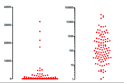
•When the geometric standard deviation is high, the lognormal distribution is asymmetrical. Lots of values are very similar, while a small fraction of the values are much larger. You can see this in the left panel of the graph below.

•When the geometric standard deviation has a low value (say less than 1.3), the asymmetry is hard to appreciate unless the sample size is huge.
•When plotted on a logarithmic axis, as shown on the right panel of the graph above, the distribution is symmetrical.
•If you are not aware of lognormal distributions, you might be tempted to remove the highest four values in the example above as outliers, since they look like they are not part of the overall distribution. If you run the values through an outlier detection algorithm that assumes sampling from a Gaussian distribution, outliers will probably be identified (the highest four values in the example above.
•If you try to compare means with a t test or ANOVA, you are likely to find that the P value is high and the confidence intervals are wide. T tests and ANOVA assume that the values were sampled from a Gaussian distribution. You will lose power if you try to use those methods to compare means of data set sampled from a lognormal distribution.
•The logarithm of all the values from a lognormal distribution is Gaussian.
How to cope with lognormal distributions
Analyzing data from a lognormal distribution is easy. Simply transform the data by taking the logarithm of each value. These logarithms are expected to have a Gaussian distribution, so can be analyzed by t tests, ANOVA, etc.
Starting with version 10.5, Prism offers lognormal versions of t-tests and one-way ANOVA. Check the option to assume sampling from lognormal distributions, and these tests compare geometrical means, and compute the ratio of geometric means (rather than the differences between arithmetic means).
How to learn more about lognormal distributions
This long article explains how to think about and analyze lognormal data.
HJ Motulsky, T Head, PBS Clarke, 2025, Analyzing Lognormal Data: A Nonmathematical Practical Guide. Pharmacological Reviews, Volume 77, Issue 3, 100049