A logarithmic X axis is useful when the X values are logarithmically spaced
The X axis usually plots the independent variable – the variable you control. If you chose X values that are constant ratios, rather than constant differences, the graph will be easier to view on a logarithmic axis.
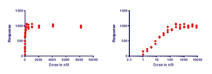
The two graphs below show the same data. X is dose, and Y is response. The doses were chosen so each dose is twice the previous dose. When plotted with a linear axis (left) many of the values are superimposed and it is hard to see what’s going on. With a logarithmic axis (right), the values are equally spaced horizontally, making the graph easier to understand.
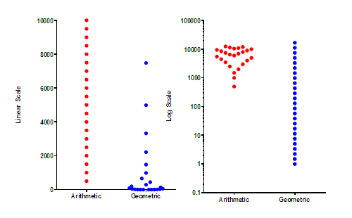
A logarithmic axis is useful for plotting ratios
Ratios are intrinsically asymmetrical. A ratio of 1.0 means no change. All decreases are expressed as ratios between 0.0 and 1.0, while all increases are expressed as ratios greater than 1.0 (with no upper limit).
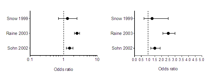
On a log scale, in contrast, ratios are symmetrical. A ratio of 1.0 (no change) is halfway between a ratio of 0.5 (half the risk) and a ratio of 2.0 (twice the risk). Thus, plotting ratios on a log scale (as shown below) makes them easier to interpret. The graph below plots odds ratios from three case‐control retrospective studies, but any ratio can benefit from being plotted on a log axis.
The graph above was created with the outcome (the odds ratio) plotted horizontally. Since these values are something that was determined (not something set by the experimenter), the horizontal axis is the Y axis even though it is horizontal.
A logarithmic axis linearizes compound interest and exponential growth
The graphs below plot exponential growth, which is equivalent to compound interest. At time = 0.0, the Y value equals 100. For each increment of 1.0 on the X axis, the value plotted on the Y axis equals 1.1 times the prior value. This is the pattern of cell growth (with plenty of space and nutrients), and is also the pattern by which an investment (or debt) grows over time with a constant interest rate.
The graph on the right is identical to the one on the left, except that the Y axis has a logarithmic scale. On this scale, exponential growth appears as a straight line. Exponential growth has a constant doubling time. For this example, the Y value (cell count, value of investment) doubles for every time increment of 7.2657.
Exponential decay is also linearized on a logarithmic axis, but only when the decay eventually decays to zero.