
Nonlinear regression: Dependency and ambiguous fits
Overview
When you fit a model with two or more parameters, they can be interwined or even redundant. Prism 5 can quantify the degree to which parameters are intertwined either by a reporting the covariance of each parameter with every other parameter (covariance matrix) or by reporting the dependency of each parameter with the others. Choose either or both on the Diagnostics tab of the Prism 5 nonlinear regression dialog.
The dependency is expressed as a fraction (0.0 to 1.0) and has a high value when parameters of the model are redundant. If the dependency of any parameter is greater than 0.9999, then Prism labels the entire fit as "ambiguous" and reports the confidence interval for the ambiguous parameters as "very wide" (and reports no numerical confidence interval).
The term and definition of "dependency" was not created by GraphPad, but the use of the term "ambiguous" for fits with high dependency is unique to GraphPad.
Interpreting dependency
The value of dependency always ranges from 0.0 to 1.0.
A dependency of 0.0 is an ideal case when the parameters are entirely independent (mathematicians would say orthogonal). In this case the increase in sum-of-squares caused by changing the value of one parameter cannot be reduced at all by also changing the values of other parameters. This is a very rare case.
A dependency of 1.0 means the parameters are redundant. After changing the value of one parameter, you can change the values of other parameters to reconstruct exactly the same curve. In this case, the confidence intervals will be very wide, and the results will not be helpful. If the dependency equals 1.0, you can probably rewrite the model using fewer parameters.
With experimental data, of course, the value lies between 0.0 and 1.0. How high is too high? Obviously, any rule-of-thumb is arbitrary. But dependency values up to 0.90 and even 0.95 are not uncommon, and are not really a sign that anything is wrong.
A dependency greater than 0.99 is really high, and tells you that something is wrong. This means that you can create essentially the same curve, over the range of X values for which you collected data, with several sets of parameter values. Your data simply do not define all the parameters in your model. If your dependency is really high, ask yourself these questions:
- Can you fit to a simpler model?
- Would it help to collect data over a wider range of X, or at closer spaced X values? It depends on the meaning of the parameters.
- Can you collect data from two kinds of experiments ,and fit the two data sets together using global fitting?
- Can you constrain one of the parameters to have a constant value based on results from another experiment?
Not all programs (or books) define dependency in exactly the same way. Some calculate it from the VIF (Variance Inflation Factor) and others do it as we did above but without the correction for degrees of freedom. So different programs might produce slightly different values for dependency. With all definitions, you'll interpret a really high dependency in the same way.
Ambiguous fits
When the dependency is >0.9999, Prism 5 precedes the parameter value with a squiggle, ~. It also labels the results 'ambiguous'. This is an arbitrary cutoff. The term 'ambiguous' is unique to Prism, but the concept is not unique. See an example of an ambiguous fit.
How dependency is calculated
This is best understood via an example. This example is an exponential decay (taken from pages 128-130 of the MLAB Applications Manual, www.civilized.com). If you want to follow the example yourself, download the data as a text file.
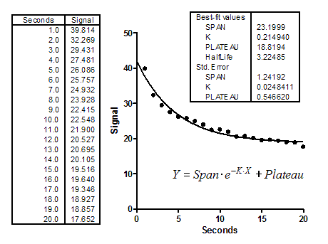
We'll focus on the rate constant, K. The best fit value is 0.2149 sec-1, which corresponds to a half-life of 3.225 seconds. Its SE is 0.0248 sec-1, which can be used to compute the confidence interval of 0.1625 to 0.2674 sec-1.
It is clear that the parameters are not independent. If you forced K to have a higher value (faster decay), the curve would get further from the points. But you could compensate a bit by starting the curve at a higher value and ending at a lower one (increase Span and decrease Plateau). The SE values of the parameters depend on one another.
Let's fix Span and Plateau to their best fit values, and ask nonlinear regression to fit only the rate constant K. This won't change the best fit value, of course, since we fixed Span and Plateau to their best-fit values. But the SE of K is lower now, equal to 0.008605. This makes sense. Changing the value of K has a bigger impact on goodness-of-fit (sum-of-squares) when you fix the Span and Plateau than it does when you allow the values of Span and Plateau to also change to compensate for the change in K.
The lower value of the SE of K when you fix the other parameters tells you that the uncertainty in K is dependent on the other parameters. We want to quantify this by computing the dependency.
Before we can compare the two SE values, we have to correct for a minor problem. When computing the SE, the program divides by the square root of the number of degrees of freedom (df). For each fit, df equals the number of data points minus the number of parameters fit by the regression. For the full fit, df therefore equals 20 (number of datapoints) minus 3 (number of parameters) or 17. When we held the values of Plateau and Span constant, there was only one parameter, so df=19. Because the df are not equal, the two SE values are not quite comparable. The SE when other parameters were fixed is artificially low. This is easy to fix. Multiply the SE reported when two of the parameters were constrained by the square root of 19/17. This corrected SE equals 0.00910.
Now we can compute the dependency. It equals 1.0 minus the square of the ratio of the two (corrected) SE values. So the dependency for this example equals 1.0-(0.0091/0.0248)2, or 0.865. Essentially, this means that 86.5% of the variance in K is due to is interaction with other parameters.
Each parameter has a distinct dependency (unless there are only two parameters). The dependency of Span is 0.613 and the dependency of Plateau is 0.815.
The origin of the idea of dependency
There appears to be no paper to cite regarding the first use of dependency. The idea of dependency apparently was developed by Dick Shrager at the NIH, and then enhanced by Gary Knott. MLAB was the first software to compute dependency, and it is explained well in the MLAB manual. GraphPad Prism simply implements the method as it is explained there. (I learned this history in an email from Gary Knott in 2007). Here is an early paper that discusses the basic ideas of dependency, but it is defined differently (ranging from 1 to infinity, rather than 0 to 1, and the math is not fully explained.