Repeated measures ANOVA, sphericity and compound symmetry

This page was written for people using Prism 5. If you use Prism 6, read here instead. 

Defining sphericity and compound symmetry

One of the assumptions of repeated measures ANOVA is called sphericity or circularity (the two are synonyms). 

Here is the table of sample data from Prism 5 (choose a Column table, and then choose sample data for repeated measures one-way ANOVA).

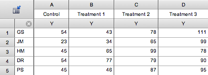
Each row represents data from one subject identified by the row title. Each column represents a different treatment. In this example, each of five subjects was given four sequential treatments. 

The assumption of sphericity states that the variance of the differences between treatment A and B equals the variance of the difference between A and C, which equals the variance of the differences between  A and D, which equals the variance of the differences between B and D...   Like all statistical assumptions, this assumption pertains to the population from which the data were sampled, and not just to this particular data set. 

This is easier to see on a graph:

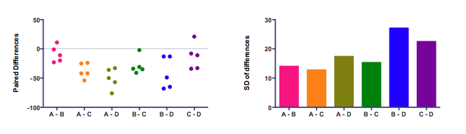
The left panel shows the differences. Each of the six columns represents the difference between two treatments. There are five subjects, so there are five dots for each difference.

Bar graphs usually plot means. Not here! The graph on the right plots the standard deviations. The assumption of sphericity is that the data were sampled from populations where these standard deviations are identical. (Most statistics books talk about variance, which is the square of the standard deviation. If the standard deviations are equal, so are the variances.) The standard deviations in the right panel above are not identical. That doesn't really matter.  The assumption is about the population of values. In any particular samples, you expect some variation. Here the variation among the standard deviations is fairly small. If the standard deviations varied a whole lot, the assumption of sphericity would be badly violated and the repeated measures results would be wrong (unless they corrected for the lack of sphericity).

You might be surprised that the differences between nonadjacent columns are considered. Why should the difference between A and C matter? Or between A and D? The answer is that ANOVA  pays no attention to the order of the groups. Repeated measures ANOVA treats each row of values as a set of matched values. But the order of the treatments is simply not considered by ANOVA, not a bit. If you randomly scrambled the treatment order of all subjects, the ANOVA results wouldn't change  (unless you choose a post test for trend). 

When you read about this topic, you will also encounter the term  compound symmetry, which is based on the covariance matrix of the raw data (without computing paired differences).  If the assumption of compound symmetry is valid for a data set, then so is the assumption of sphericity (it is possible, but rare, for data to violate compound symmetry even when the assumption of sphericity is valid). 

 

Violations of the assumption

First separate the concepts of repeated measures data from randomized block data.

In a randomized block experiment, matched subjects (or whatever) are given alternative treatments at one time, but no one subject gets repeated treatments. Randomized block experiments are unlikely to violate sphericity.

In a repeated measures experiment each subject is given sequentially different treatments (or just measured sequentially to see the effect of time). If measurements are made too close together, any random effect that causes a particular value to be high (or low) may not wash away or dissipate before the next measurement, which would lead to circularity problems. To avoid violating the assumption, wait long enough between treatments so the subject is essentially the same as before the treatment. When possible, also randomize the order of treatments.

Effects of violating the assumption

There is a simple calculations you can do by hand to get a sense of how serious violations of the sphericity assumption could be matter. Here is the ANOVA table as reported by Prism:

Source of Variation	SS	df	MS
Treatment (between columns)	8417	3	2806
Individual (between rows)	949.3	4	237.3
Residual (random)	2136	12	178.0
Total	11503	19

The ratio of the MS for variation between treatments (columns) divided by the MS for random variation equals the F ratio, which is  2806/237.3 or 15.76. The degrees of freedom are shown next to the corresponding MS values. You can use the free GraphPad Quickcalc to compute the exact P value. Or use this Excel formula: =FDIST(15.76,3,12). The P value is 0.000183, which Prism reports as 0.0002.

If the sphericity assumption is violated, this P value will be too low.  But it is easy to find the worst case. How large would the P value be if the assumption of compound symmetry were grossly violated? A method called the lower-bound adjustment  computes this. Compute the P value for the same F ratio, but reduce the degrees of freedom to 1 for the numerator, and n-1 for the denominator (where n is the number of subjects). For this example, we can find the P value using this Excel formula: =FDIST(15.76,1,4). This adjusted (lower bound) P value is 0.0165. 

In other words, the true P value (which we didn't calculate) is between 0.0002 (assuming compound symmetry) and 0.0165 (assuming horrendous violations of compound symmetry). Since these are all tiny P values, we can be confident of the conclusion, even without explicitly testing for violations of compound symmetry

Quantifying violations of sphericity

The degree of violation of the sphericity assumption can be quantified by the value epsilon. 

Correcting for violations of sphericity

Some programs measure the extent to which the compound symmetry assumption is violated, and compute P values which take into account this violation. Read about these methods of in Chapter 11 of Maxwell and Delaney (reference below).  

There are two such methods. Maxwell and Delaney recommend the method of Geisser and Greenhouse. That P value is 0.00307. The other  method was developed by Huynh and Feldt. For this example, this P value is 0.000211.  (Both these values were computed by NCSS). 

Both these P values are computed using the same F ratio, but with adjustments to the numbers of degrees of freedom (with different adjustments using the two methods). 

Learn more:

The Bluffer's Guide to Sphericity,  This is a great explanation written by Andy Field at the University of Sussex.