Introduction
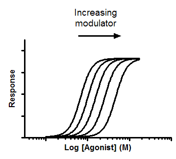
A competitive inhibitor competes for agonist binding to a receptor, and shifts the dose-response curve to the right without changing the maximum response. By fitting all the curves globally, you can determine the affinity of the competitive inhibitor.
Step by step
1.Create an XY data table with subcolumns to match your experimental design.
2.Enter the logarithm of the concentration of the agonist ligand into X. For example, if a concentration is 1nM, enter -9. Don't enter 1e-9.
3.Enter response into Y in any convenient units. Enter data with no inhibitor into column A. Enter data collected with a constant concentration of inhibitor into column B. Repeat, if you have data, for column C, D, E, ..., each with a different concentration of inhibitor.
4.Enter the inhibitor concentration in molar as the column titles of the data table. If the concentration is 1nM enter '1e-9' or '0.00000001' into the column titles. Don't enter '-9'. Don't forget to enter '0' as the column title for data set A, since these are the control data with no inhibitor. These values entered into the column title are used in the analyis; they are more than just labels, so need to be entered in the correct format.
5.From the data table, click Analyze, choose nonlinear regression, and choose the panel of equations: Dose-Response -- Special. Then choose Gaddum/Schild EC50 shift.
6.Consider constraining the parameters HillSlope and SchildSlope to their standard values of 1.0. This is especially useful if you don't have many data points, and therefore cannot fit these parameters.
Notes on units
•This equation was written so the X values are entered as logarithm of concentration of the agonist, while the column titles are entered as concentration of antagonist. This is simply the way this equation was written. It would be easy enough to clone the equation and write it with different conventions if you wanted to.
•The EC50 is reported in the antilog of the units you used to enter X values. If you entered X as log(molar), then the EC50 will be in molar. If you entered X values as log(dose in milligrams), then the EC50 will be in milligrams.
•The pA2 is the negative logarithm of the concentration of antagonist needed to shift the curve by a factor of 2. That concentration is in the same units you used to enter the antagonist concentration into the column titles. If you entered concentration in nM into the column titles, the pA2 is the negative logarithm of nM. If you entered concentration as a dose in mg/kg, then the pA2 is the negative logarithm of mg/kg.
•If you want to transform the pA2 to a concentration, first flip the sign (multiply by -1) and then take the antilog (ten to that power). If you also do so for the confidence limits, note that flipping the sign also changes the order of the limits, so the "lower" confidence limit is actually the upper limit, and the "upper" limit is actually the lower limit.
Model
EC50=10^LogEC50
Antag=1+(B/(10^(-1*pA2)))^SchildSlope
LogEC=Log(EC50*Antag)
Y=Bottom + (Top-Bottom)/(1+10^((LogEC-X)*HillSlope))
Interpret the parameters
EC50 is the concentration of agonist that gives half maximal response in the absence of inhibitor. Prism reports both the EC50 and its log. The logEC50 is in the same units you used to enter the X values. The EC50 is in the antilog of those units.
pA2 is the negative logarithm of the concentration of antagonist needed to shift the dose response curve by a factor of 2. If the HillSlope and SchildSlope are fixed to 1.0, it is the pKb, the negative log of the equilibrium dissociation constant (Molar) of inhibitors binding to the receptors. The units are the negative log of whatever units you used to enter concentrations as column titles on the data table.
HillSlope describes the steepness of the family of curves. A HillSlope of 1.0 is standard, and you should consider constraining the Hill Slope to a constant value of 1.0.
SchildSlope quantifies how well the shifts correspond to the prediction of competitive interaction. If the competitor is competitive, the SchildSlope will equal 1.0. You should consider constraining SchildSlope to a constant value of 1.0. antagonist term, [B], is now raised to the power S, where S denotes the Schild slope factor. If the shift to the right is greater than predicted by competitive interactions, S will be greater than 1. If the rightward shift is less than predicted by competitive interaction, then S will be less than 1.
Top and Bottom are plateaus in the units of the Y axis.
Notes:
•All six of these are shared among all the data sets, so you will only see one best fit value for each parameter, not one for each data set.
•Prism does not report the EC50 for each curve, only the EC50 for the first curve (the one without any antagonist).
•The variable B in the model is defined to be a data set constant whose value comes from the column titles. The results page will show these values of B. Make sure they are the concentration of antagonist used in each data set (and not the log of concentrations).
When is the Schild model valid?
Colquhoun (1) has shown that the Schild model is valid whenever you can make these assumptions:
•The antagonist, B, is a true antagonist that, alone, does not change the conformation of the receptor.
•Binding of agonist, A, and antagonist, B, is mutually exclusive at every binding site.
•B has the same affinity for every binding site.
•The observed response is the same if the occupancy of each site by A is the same, regardless of how many sites are occupied by B.
•Measurements are made at equilibrium.
1. Colquhoun, D.. Why the Schild method is better than Schild realised. Trends Pharmacol Sci (2007) vol. 28 (12) pp. 608-14