What are planned comparisons?

The term planned comparison is used when you focus in on a few scientifically sensible comparisons. You don't do every possible comparison. And you don't decide which comparisons to do after looking at the data. Instead, you decide -- as part of the experimental design -- to only make a few comparisons.

Some statisticians recommend not correcting for multiple comparisons when you make only a few planned comparisons. The idea is that you get some bonus power as a reward for having planned a focussed study.

Prism always corrects for multiple comparisons, without regard for whether the comparisons were planned or post hoc. But you can get Prism to do the planned comparisons for you once you realize that a planned comparison is identical to a Bonferroni corrected comparison for selected pairs of means, when there is only one pair to compare.

Example data with incorrect analysis

In the graph below, the first column shows control data, and the second column shows data following a treatment. The goal of the experiment is to see if the treatment changes the measured activity (shown on the Y axis). To make sure the vehicle (solvent used to dissolve the treatment) isn't influencing the result, the experiment was performed with another control that lacked the vehicle (third column). To make sure the experiment is working properly, nonspecific (blank) data were collected and displayed in the fourth column.

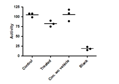
Here are the results of one-way ANOVA and Tukey multiple comparison tests comparing every group with every other group.

The overall ANOVA has a very low P value, so you can reject the null hypothesis that all data were sampled from groups with the same mean. But that really isn't very helpful. The fourth column is a negative control, so of course has much lower values than the others. The ANOVA P value answers a question that doesn't really need to be asked.

Tukey's multiple comparison tests were used to compare all pairs of means (table above). You only care about the first comparison -- control vs. treated -- which is not statistically significant (P>0.05).

These results don't really answer the question your experiment set out to ask. The Tukey multiple comparison tests set the 5% level of significance to the entire family of six comparisons. But five of those six comparisons don't address scientifically valid questions. You expect the blank values to be much lower than the others. If that wasn't the case, you wouldn't have bothered with the analysis since the experiment hadn't worked. Similarly, if the control with vehicle (first column) was much different than the control without vehicle (column 3), you wouldn't have bothered with the analysis of the rest of the data. These are control measurements, designed to make sure the experimental system is working. Including these in the ANOVA and post tests just reduces your power to detect the difference you care about.

Example data with planned comparison

Since there is only one comparison you care about here, it makes sense to only compare the control and treated data.

From Prism's one-way ANOVA dialog, choose the Bonferroni comparison between selected pairs of columns, and only select one pair.

The difference is statistically significant with P<0.05, and the 95% confidence interval for the difference between the means extends from 5.826 to 39.51.

When you report the results, be sure to mention that your P values and confidence intervals are not corrected for multiple comparisons, so the P values and confidence intervals apply individually to each value you report and not to the entire family of comparisons.

In this example, we planned to make only one comparison. If you planned to make more than one comparison, choose the Fishers Least Significant Difference approach to performing multiple comparisons. When you report the results, be sure to explain that you are doing planned comparisons so have not corrected the P values or confidence intervals for multiple comparisons.

Example data analyzed by t test

The planned comparisons analysis depends on the assumptions of ANOVA, including the assumption that all data are sampled from groups with the same scatter. So even when you only want to compare two groups, you use data in all the groups to estimate the amount of scatter within groups, giving more degrees of freedom and thus more power.

That assumption seems dubious here. The blank values have less scatter than the control and treated samples. An alternative approach is to ignore the control data entirely (after using the controls to verify that the experiment worked) and use a t test to compare the control and treated data. The t ratio is computed by dividing the difference between the means (22.67) by the standard error of that difference (5.27, calculated from the two standard deviations and sample sizes) so equals 4.301. There are six data points in the two groups being compared, so four degrees of freedom. The P value is 0.0126, and the 95% confidence interval for the difference between the two means ranges from 8.04 to 37.3.

How planned comparisons are calculated

First compute the standard error of the difference between groups 1 and 2. This is computed as follows, where N1 and N2 are the sample sizes of the two groups being compared (both equal to 3 for this example) and MSresidual is the residual mean square reported by the one-way ANOVA (80.0 in this example):

For this example, the standard error of the difference between the means of column 1 and column 2 is 7.303.

Now compute the t ratio as the difference between means (22.67) divided by the standard error of that difference (7.303). So t=3.104. Since the MSerror is computed from all the data, the number of degrees of freedom is the same as the number of residual degrees of freedom in the ANOVA table, 8 in this example (total number of values minus number of groups). The corresponding P value is 0.0146.

The 95% confidence interval extends from the observed mean by a distance equal to SE of the difference (7.303) times the critical value from the t distribution for 95% confidence and 8 degrees of freedom (2.306). So the 95% confidence interval for the difference extends from 5.826 to 39.51.