A single Prism analysis smooths a curve and/or converts a curve to its derivative or integral.
Finding the derivative or integral of a curve
The first derivative is the steepness of the curve at every X value. The derivative is positive when the curve heads uphill and is negative when the curve heads downhill. The derivative equals zero at peaks and troughs in the curve. After calculating the numerical derivative, Prism can smooth the results, if you choose.
The second derivative is the derivative of the derivative curve. The second derivative equals zero at the inflection points of the curve.
The integral is the cumulative area between the curve and the line at Y=0, or some other value you enter.
Notes:
•Prism cannot do symbolic algebra or calculus. If you give Prism a series of XY points that define a curve, it can compute the numerical derivative (or integral) from that series of points. But if you give Prism an equation, it cannot compute a new equation that defines the derivative or integral.
•This analysis integrates a curve, resulting in another curve showing cumulative area. Don't confuse with a separate Prism analysis that computes a single value for the area under the curve.
Smoothing a curve
If you import a curve from an instrument, you may wish to smooth the data to improve the appearance of a graph. Since you lose data when you smooth a curve, you should not smooth a curve prior to nonlinear regression or other analyses.
Prism gives you two ways to adjust the smoothness of the curve. You choose the number of neighboring points to average and the 'order' of the smoothing polynomial. Since the only goal of smoothing is to make the curve look better, you can simply try a few settings until you like the appearance of the results. If the settings are too high, you lose some peaks which get smoothed away. If the settings are too low, the curve is not smooth enough. The right balance is subjective -- use trial and error.
The results table has fewer rows than the original data.
Don't analyze smoothed data
Smoothing a curve can be misleading. The whole idea is to reduce the "fuzz" so you can see the actual trends. The problem is that you can see "trends" that don't really exist. The three graphs in the upper row below are simulated data. Each value is drawn from a Gaussian distribution with a mean of 50 and a standard deviation of 10. Each value is independently drawn from that distribution, without regard to the previous values. When you inspect those three graphs, you see random scatter around a horizontal line, which is exactly how the data were generated.
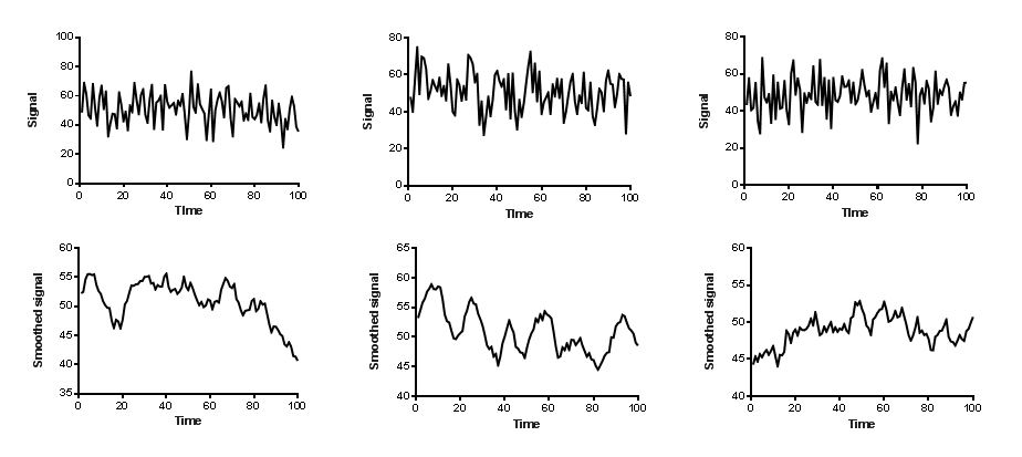
The bottom three graphs above show the same data after smoothing (averaging 10 values on each side, and using a second order smoothing polynomial). When you look at these graphs, you see trends. The first one tends to trend down. The second one seems to oscillate in a regular way. The third graph tends to increase. All these trends are artefacts of smoothing. Each graph shows the same data as the graph just above it.
Smoothing the data creates the impression of trends by ensuring that any large random swing to a high or low value is amplified, while the point-to-point variability is muted. A key assumption of correlation, linear regression and nonlinear regression is that the data are independent of each other. With smoothed data, this assumption is not true. If a value happens to be super high or low, so will the neighboring points after smoothing. Since random trends are amplified and random scatter is muted, any analysis of smoothed data (that doesn't account for the smoothing) will be invalid.
Mathematical details
•The first derivative is calculated as follows (x, and Y are the arrays of data; x' and y' are the arrays that contain the results).
x'[i] = (x[i+1] + x[i]) / 2
y' at x'[i] = (y[i+1] - y[i]) / (x[i+1] - x[i])
•The second derivative is computed by running that algorithm twice, to essentially compute the first derivative of the first derivative.
•Prism uses the trapezoid rule to integrate curves. The X values of the results are the same as the X values of the data you are analyzing. The first Y value of the results equals a value you specify (usually 0.0). For other rows, the resulting Y value equals the previous result plus the area added to the curve by adding this point. This area equals the difference between X values times the average of the previous and this Y value.
•Smoothing is done by the method of Savistsky and Golay (1).
•If you request that Prism both both smooth and convert to a derivative (first or second order) or integral, Prism does the steps sequentially. First it creates the derivative or integral, and then it smooths.
Reference
1. A. Savitzky and M.J.E. Golay, (1964). Smoothing and Differentiation of Data by Simplified Least Squares Procedures. Analytical Chemistry 36 (8): 1627–1639