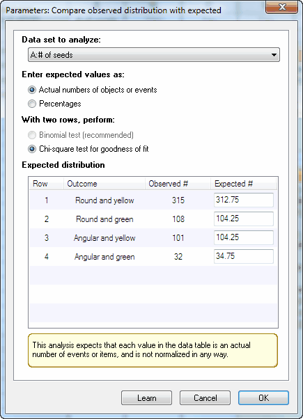
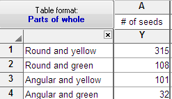
This analysis compares the distribution you entered into a parts-of-whole table (observed distribution) with a theoretical distribution you enter into the dialog (expected distribution).

1. Enter the data onto a parts-of-whole table

Enter the actual number of objects or events. The results will be meaningless if you enter normalized values, rates or percentages. These are actual data from one of Mendel's famous experiments. I obtained the data from H.  Cramer. Mathematical methods of statistics. Princeton University Press, 1999.

2. Enter the expected values

Click Analyze, and choose Compare observed distribution with expected in the Parts of whole section. These values were computed by multiplying a proportion predicted by Hardy-Weinberg Mendelian genetics (9/16 or 0.5625 for the first category) times the number of peas used in the experiment. You can also enter the percentages directly by selecting an option on the dialog.

Enter the expected values. You can choose to enter the actual number of objects or events expected in each category, in which case the total of the expected values must equal the total of the observed data you entered on the data table. Or you can choose to enter percentages, in which case they must total 100. In either case, it is ok to enter fractional values.

In this example, the expected values are not integers. That's ok. That is the average expectation if you did a large number of experiments. In any one experiment, of course, the number of peas of each category must be an integer. These values are computed based on Mendelian genetics. For example, the theory predicts that 9/16 of peas would be in the first category. Multiply that fraction by the total number of peas used in this experiment to get the expected values.

3. Choose the test

If you entered more than two rows of data (as in the example above), you'll have no choice. Prism will perform the chi-square goodness-of-fit test.

If you entered only two rows of data, you can also choose the binomial test, which we strongly recommend. With only two categories, the chi-square test reports P values that are too small. This is a huge issue with small data sets, but the discepancy exists even with sample sizes in the hundreds. Use the binomial test.

4. Interpret the P value

The results table summarizes the data, reports the value of chi-square and its df (if you picked the chi-square test), and states the P value. The null hypothesis is that the observed data are sampled from a populations with the expected frequencies. The P value answers this question:

Assuming the theory that generated the expected values is correct, what is the probability of observing such a large discrepancy (or larger) between observed and expected values?

A small P value is evidence that the data are not sampled from the distribution you expected. In this example, the P value is large  (0.93) so the data provide no evidence of a discrepancy between the observed data and the expected values based on theory.