Prism provides a number of important options for the multiple t test (and nonparametric tests) analysis, allowing you to choose from one of seven different tests to perform for each row of the data table.

The experimental design tab

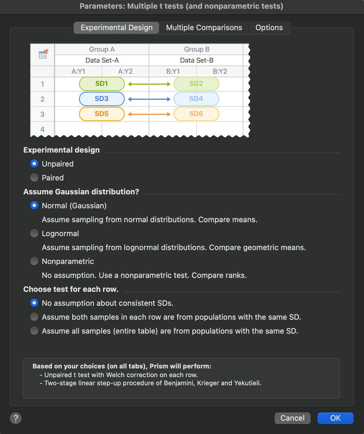
The first tab of the Parameters: Multiple t tests (and nonparametric tests) analysis dialog presents a number of options that allow you to specify the type of analysis to perform by answering three questions:

1.Are the data paired or unpaired?

2.Will the tests assume a Gaussian (Normal) distribution?

3.Based on the answers to the previous two questions, which specific test should Prism perform?

Experimental Design: Are the data paired or unpaired?

This first question pertains to the relationship of the data within each main group being compared. If the option "Paired" is selected, this means that data in the first subcolumn of each main column is paired or matched, the data in the second subcolumn of each main column is paired or matched, and so on. Examples of when you may choose this option include:

•Measurements were performed on the same subject at different times (for example, before and after a treatment)

•Measurements were performed on individuals that were recruited or matched as pairs based on characteristics such as age, ethnic group, or disease severity. In this situation, one individual may receive one treatment while the other receives an alternative treatment (or serves as a control)

•You run a laboratory experiment several times, each time with a control and treated preparation handled in parallel. This may be important if uncontrollable experimental conditions vary slightly between preparations

•You measure a variable in individuals with some inherent pairing, such as twins or child/parent pairs

Note that matching should be determined by the experimental design, and should definitely not be based on the variable being analyzed. For example, if you are comparing measurements of blood pressure in two groups, it is OK to match individuals on age or body weight, but it is not OK to match based on their recorded blood pressure.

Assume Gaussian distribution?

Nonparametric tests are not based on the assumption that the data are sampled from a Gaussian distribution. This may seem like an advantage (reducing the number of assumptions required about the data), however nonparametric tests have less power. Moreover, deciding when to use a nonparametric test is not straightforward.

Choose test for each row

Based on the options selected in the previous two sections, the final decision to make on the Experimental Design tab of the analysis parameters dialog is which specific test to perform. There are seven total tests that can be performed for each row, some of which have additional options to consider. Each test and the options available in this final section are described below.

1.Unpaired, parametric test. Selecting this combination of options in the previous two sections results in making one final decision about the standard deviation of each group in the analyses.

oThe first choice makes no assumptions about the standard deviations of the populations from which the data in any row or column were sampled from. By selecting this option, Prism will perform the unequal variance unpaired t test (sometimes called the unpaired t test with Welch's correction)

oThe next choice is to assume that - for each row - the data of both groups were sampled from populations with the same standard deviation (in other words, the SD of the population from which data in one row in the first column were selected is the same as the SD of the population from which the data in the same row of the second column were selected). This will perform a standard, unpaired t test for each row with individual variances estimated for each row, and is the default choice for an unpaired, parametric test

oThe final choice in this section allows for the assumption that all data (all groups on all rows) were sampled from populations with the SAME standard deviation. Note that this does NOT mean that your sample standard deviations must be identical. Instead, the assumption here is that the variation in the samples is random, and that all of the data from all rows comes from populations with the same standard deviation. This is the assumption of homoscedasticity, and results in more degrees of freedom and thus more power. With this option, Prism will perform an unpaired t test with a single pooled variance

2.Paired, parametric test.  Selecting this combination of options in the previous two sections results in making one final decision regarding which test Prism will perform (which null hypothesis Prism will test)

oPaired t test. The null hypothesis for this test is that the average of the differences between each of the pairs is zero

oRatio t test. The null hypothesis for this test is slightly more complicated. Briefly, the null hypothesis of this test is that the average of the logarithms of the ratio of each pair is zero (or in other words that the ratio of each pair is 1 since log(1) = 0)

3.Unpaired, nonparametric test. Selecting this combination of options results in having to choose between one of two tests:

oMann-Whitney test. The null hypothesis for this test can be difficult to understand, and is discussed here. However, it's important to note that this test works by taking all of the data from the two groups being compared, and ordering all of these values from smallest to largest (regardless of which of the two groups the value belongs to). Then, each value is assigned a rank, starting at 1 for the lowest value, and n for the largest value (where n is the total number of values). The test then compares the average ranks of the two groups being compared.

oKolmogorov-Smirnov test. The null hypothesis of this test can be very difficult to understand, but assumes that the two groups being compared were sampled from populations with identical distributions. This test uses the cumulative distributions of the data to test for any violation of this null hypothesis (different medians, different variances, or different distributions). More information on the Kolmogorov-Smirnov test

4.Paired, nonparametric test. Selecting this combination of options results in only one possible test:

oWilcoxon matched-pairs signed rank test. This nonparametric test first calculates the differences between pairs in the two groups being analyzed, assigns ranks to the absolute value of these differences, then compares the sum of ranks in which the paired value in the first group was higher to the sum of ranks in which the paired value in the second group was higher. This is a complicated test to understand, and other pages in this guide provide more information on interpreting the results of this test.

The Multiple Comparisons tab

When performing a whole bunch of t tests at once, the goal is usually to come up with a subset of comparisons where the difference seems substantial enough to be worth investigating further. Prism offers two approaches to decide when a two-tailed P value is small enough to make that comparison worthy of further study following the multiple t tests (and nonparametric) analysis.

One approach is based on the familiar idea of statistical significance.

The other choice is to base the decision on the False Discovery Rate (FDR; recommended).  The whole idea of controlling the FDR is quite different than that of declaring certain comparisons to be "statistically significant".   This method doesn't use the term "significant" but rather the term "discovery".  You set Q, which is the desired maximum percent of "discoveries" that are false discoveries. In other words, it is the maximum desired FDR.

Of all the rows of data flagged as "discoveries", the goal is that no more than Q% of them will be false discoveries (due to random scatter of data) while at least 100%-Q% of the discoveries are true differences between population means. Read more about FDR. Prism offers three methods to control the FDR.

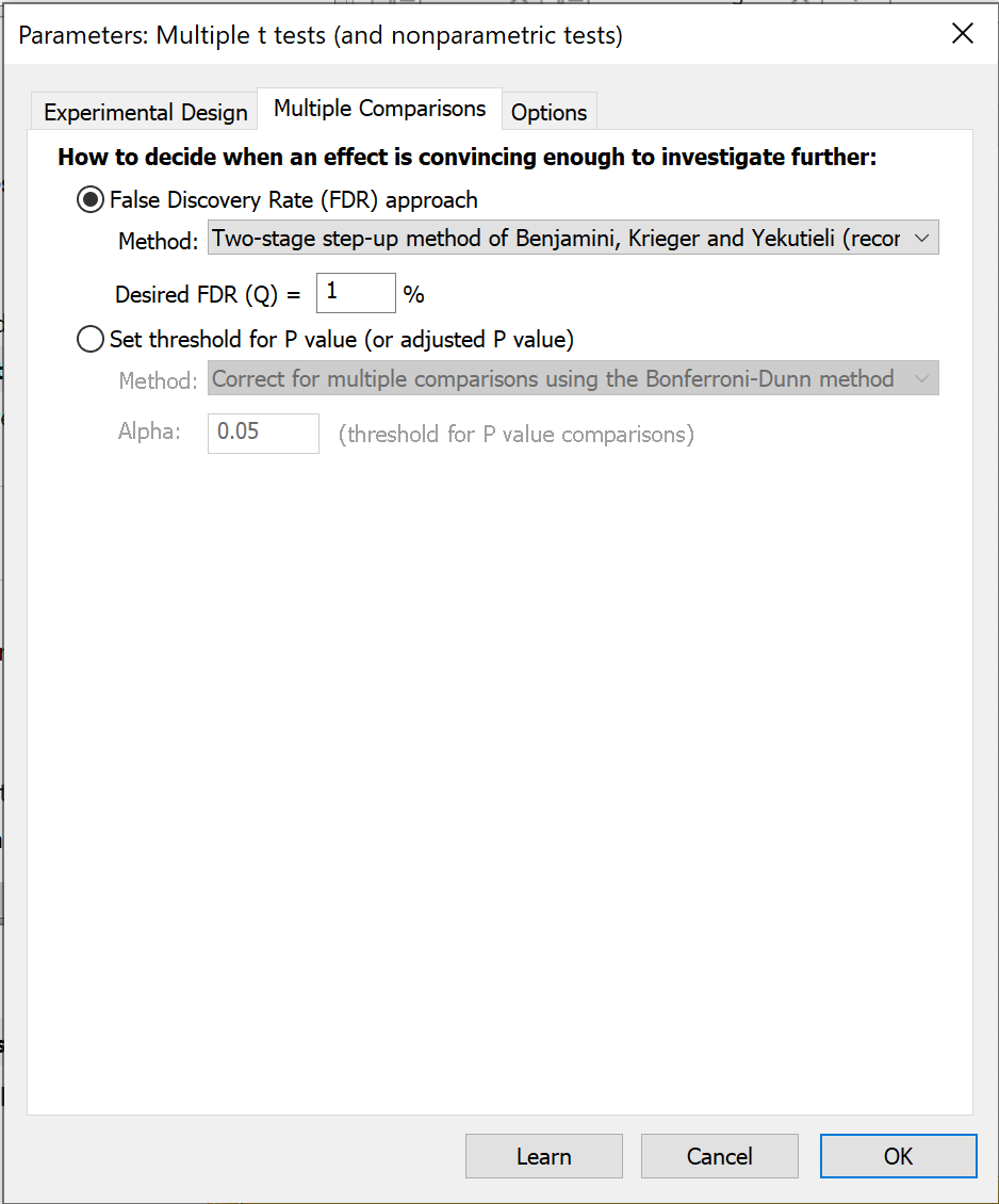
How to deal with multiple comparisons

If you chose the False Discovery Rate approach, you need to choose a value for Q, which is the acceptable percentage of discoveries that will prove to be false. Enter a percentage, not a fraction. If you are willing to accept 5% of discoveries to be false positives, enter 5 not 0.05. You also need tochoose which method to use.

If you choose to use the approach of statistical significance, you need to make an additional decision about multiple comparisons. You have four choices:

•Correct for multiple comparisons using the Holm-Šídák method (recommended).  You specify the threshold level, alpha, you want to use for the entire family of P value comparisons. This method is designed such that the specified alpha value represents the probability of obtaining a "significant" P value for one or more comparison if the null hypotheses were actually true for the comparisons of every single row.

•Correct for multiple comparisons using the Šídák-Bonferroni method (not recommended). We recommend using the Holm-Šídák method (see above) which has more power. The Šídák-Bonferroni method, often just called the Šídák method, has a bit more power than the plain Bonferroni-Dunn method (often simply called the Bonferroni approach). This is especially true when you are performing many comparisons.

•Correct for multiple comparisons using the Bonferroni-Dunn method (not recommended). The  Bonferroni-Dunn method is much simpler to understand and is better known than the Holm-Šídák method, but it has no other advantages. The primary difference between the Bonferroni-Dunn and Šídák-Bonferroni methods is that the Šídák-Bonferroni method assumes that each comparison is independent of the others, while the Bonferroni-Dunn method does not make this assumption of independence. As a result, the Šídák-Bonferroni method has slightly more power than the Bonferroni-Dunn method

•Do not correct for multiple comparisons (not recommended). Each P value is interpreted individually without regard to the others. You set a value for the significance level, alpha, often set to 0.05. This value serves as a threshold against which the P values are compared. If a P value is less than alpha, that comparison is deemed to be "statistically significant". If you use this approach, understand that you'll get a lot of false positives (you'll get a lot of "significant" findings that turn out not to be true). That's ok in some situations, like drug screening, where the results of the multiple t tests are used merely to design the next level of experimentation.

The Options tab

The third and final tab on the Parameters: Multiple t test (and nonparametric tests) analysis dialog provides a number of important controls for setting up how the results of the analysis will be reported and what sorts of visualizations Prism will generate from this analysis.

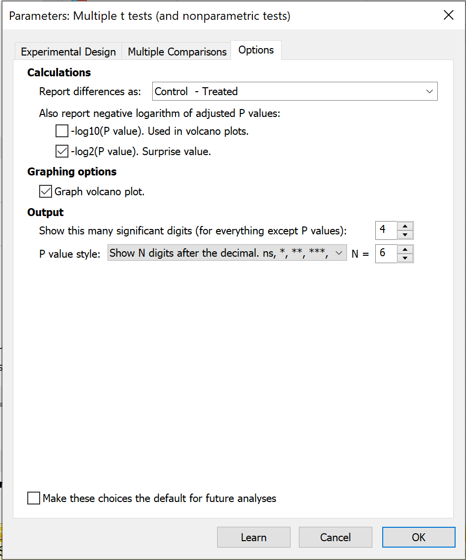
Calculations

In this section, you are able to select the order that the two groups in the analysis will be compared. For example, instead of having the differences reported as "Control - Treated" you may want to have these results reported as "Treated - Control". Note that this will not change the overall results of the test, but will only change the "sign" of the differences.

Also in this section, there is the option to report two logarithm-based transformations of the calculated P values:

•-log10(P value) - this transformation is used when creating volcano plots of the results, and this option can be used to generate a table of these results (useful to report alongside a graphed volcano plot)

•-log2(P value) - this is the base-2 logarithm of the calculated P value, and is sometimes referred to as a "Shannon information value", "Surprise value", or "S value". This simple transformation of the calculated P value provides an intuitive way of thinking about P values. Applying this transformation results in a value, S, that can be interpreted in the following way: we should be no more surprised by the obtained P value than we would be by flipping a coin S number of times and getting heads every time. As an example, let's say we had a P value of 0.125. The corresponding S value would be 3, and we should be no more surprised at obtaining a P value of 0.125 than we would be of flipping a coin three times and it landing on heads all three times (not too surprising). Now let's say we had a P value of 0.002. The corresponding S value would be ~9, and we should be no more surprised at obtaining a P value of 0.002 than we would be of flipping a coin nine times and it landing on heads every time (quite a bit more surprising!).

Graphing Options

The checkbox here (enabled by default) causes Prism to create a volcano plot of your data. The X axis is the difference between means for each row. The Y axis plots the a transformation of the P value. Specifically, it plots the negative logarithm of the P value. So if P=0.01, log(P)=-2, and -log(P)=2, which is plotted. So rows with larger differences are further to either edge of the graph and rows with smaller P values are plotted higher on the graph.

Prism automatically places a vertical grid line at X=0 (no difference) and a horizontal grid line at Y=-log(alpha). Points above this horizontal grid line have P values less than the alpha you chose.

Output

Finally on this tab, controls are available that allow you to control how many significant digits (for everything except P values) are displayed in the results of the analysis, and what style is used when reporting P values.