Looking up the strict definition for “eigenvalue” or “eigenvector” is unlikely to yield a reasonable explanation as to what these values represent unless you get into the necessary matrix algebra from which they’re calculated. Instead, let’s go back to the visual representation of our data and the first principal component identified for it:

 

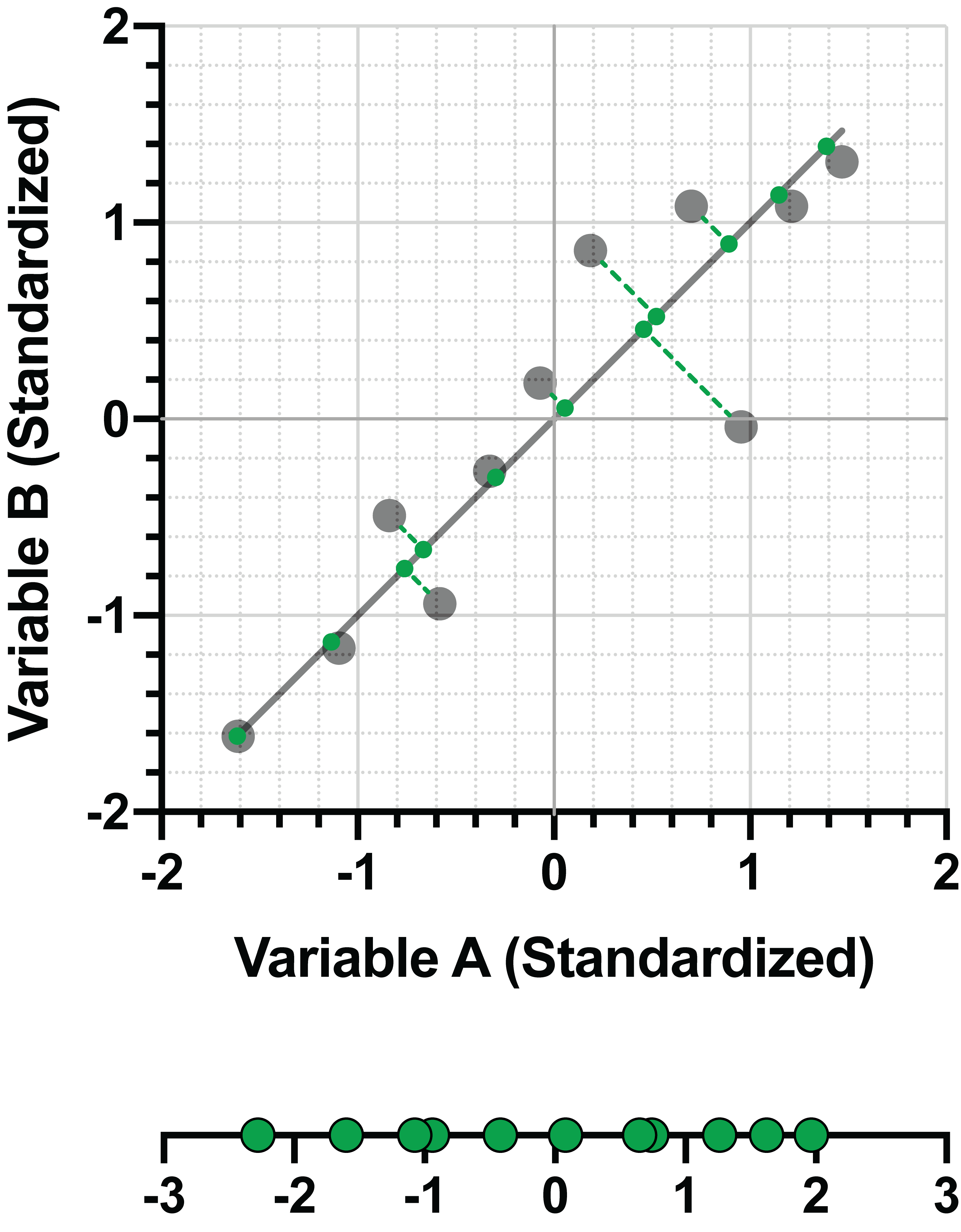
This PC was given as the linear combination:

PC1 = 0.707*(Variable A) + 0.707*(Variable B)

The coefficients, 0.707 for Variable A and 0.707 for Variable B, together represent the eigenvector for PC1. In simple terms, these values represent the “direction” of the first principal component, in the same way that a slope indicates the direction of a regression line. Starting at the coordinates (0,0) in the graph above, it can be seen that the “direction” of the line is to go to the right by 0.707 on the Variable A axis, and to go up by 0.707 on the Variable B axis. A straight line drawn between these two points will be PC1.

Advanced note: eigenvectors (like all vectors) have both direction and magnitude (like length). The direction of a vector in two-dimensional space can be defined by two values - the component of the vector in the direction of the first dimension, and the component of the vector in the second dimension. With more dimensions, a vector will require more values to fully describe it. In PCA, a single eigenvector will have one value for each of the original variables.

Why did the eigenvector end up with these strange decimal values instead of something simpler like 1 and 1? It comes down to the pythagorean theorem. In the previous example, it was shown that PC1 is the straight line that passes through the coordinates (0,0) and the coordinate (0.707, 0.707) from the eigenvector. If we were to determine the length of the line connecting these two points (also called the vector's magnitude), we’d find that it equals 1!

d = √[(0.707-0)2+(0.707-0)2]=1

*Note, the value 0.707 is a rounded value, so the above equation is off by just a bit

In fact, this is a property that is true for all eigenvectors of PCs. The length of the eigenvector is always 1, and this can be verified by finding the sum of the squares of the values of the eigenvector. Let’s look at PC2 for the same data above:

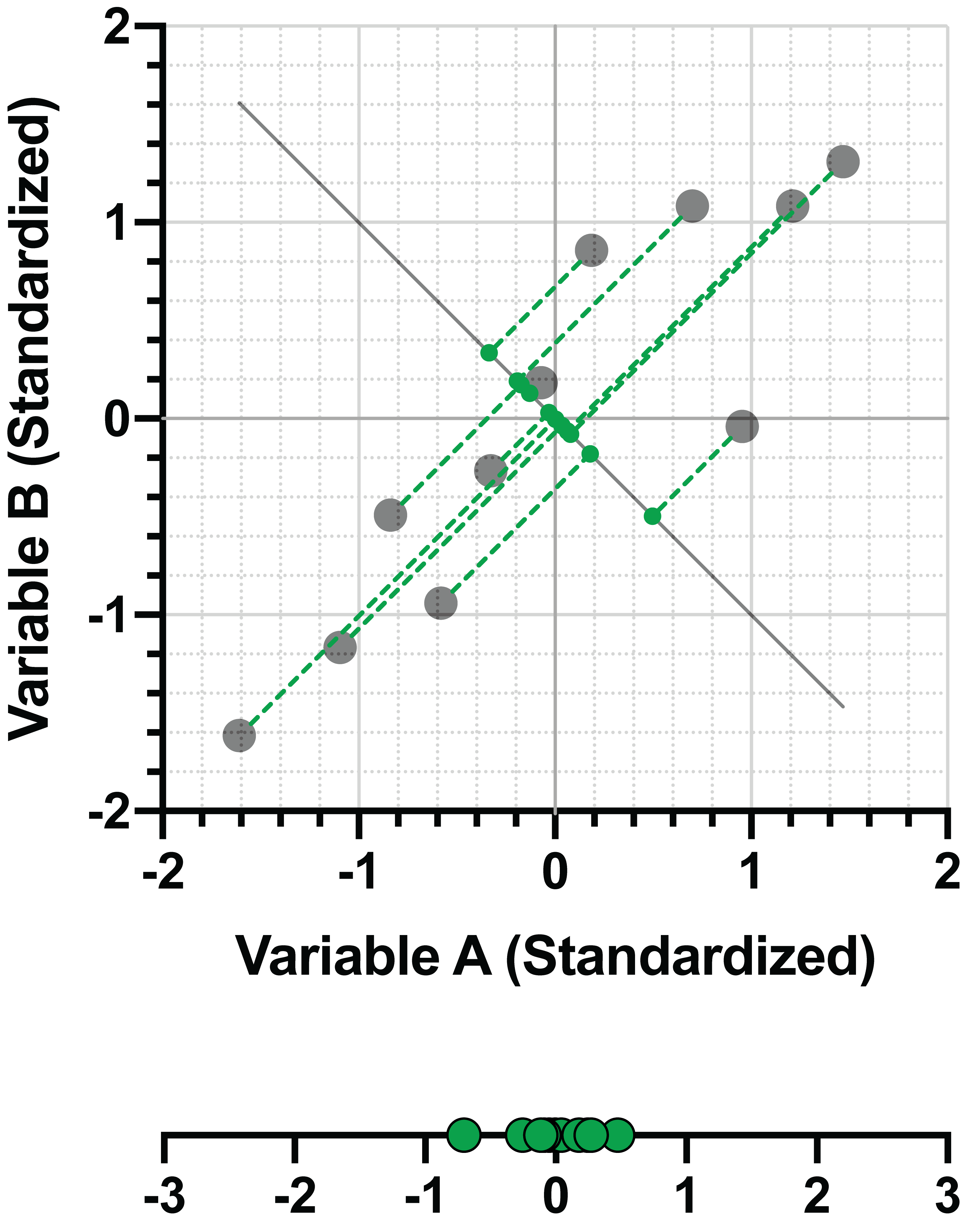
PC2 = -0.707*(Variable A) + 0.707*(Variable B)

And again,

d = √[(-0.707)2+(0.707)2]=1

So, the eigenvectors indicate the direction of each principal component. What about the eigenvalues? It turns out that these values represent the amount of variance explained by the principal component. For a set of PCs determined for a single dataset, PCs with larger eigenvalues will explain more variance than PCs with smaller eigenvalues. In this way, the eigenvalue could be considered a length of the PC to accompany the direction of the eigenvector. Note that in some situations, the loadings are used to describe this relationship between the original variables and the PCs. This section talks more about what loadings are and their relationship to eigenvectors.

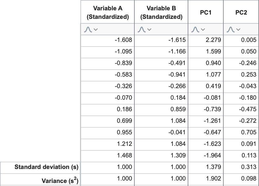
Continuing with our example, the eigenvalues for PC1 and PC2 are 1.902 and 0.098, respectively. This confirms what we said earlier about the first principal component explaining the greatest amount of variance, and each subsequent component explaining less and less total variance. To calculate these values directly, consider the “scores” that we calculated for PC1 and PC2 using the linear combinations and the standardized data.

If you calculate the standard deviation for the columns “PC1 Scores” and “PC2 Scores”, and then square those values (variance = [standard deviation]2), you get… you guessed it: 1.902 and 0.098, respectively.

Sum of eigenvalues and number of original variables

There is another interesting aspect to eigenvalues that should be discussed before moving on with component selection. Namely that - if you’re using standardized data for the analysis - the sum of eigenvalues for all PCs will equal the total number of original variables. Why?

Remember that standardizing the data results in each variable having a variance equal to 1. By extension, the total amount of variance in the dataset is equal to the total number of variables. Each PC “explains” an amount of this variance equal to its eigenvalue, but doesn’t change the overall amount of variance in the data. Since none of the variance is removed by projecting the data onto the new PCs, the sum of explained variance for all PCs must equal the total variance. Thus, the sum of eigenvalues = sum of explained variance = total variance = number of original variables.

This fact is useful when selecting a subset of PCs to achieve dimensionality reduction.