One of the primary results of Kaplan-Meier survival analysis is the survival proportions or percentages at each time point. These values are most often presented graphically, but it is sometimes useful to view the table of these results as well. The analysis results tab for these values is invisible by default. In order to view it, simply click the dropdown menu at the right side of the analysis tabs, and select it from the list.
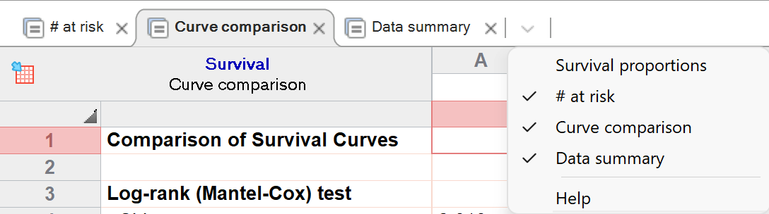
Survival proportions
Prism calculates survival proportions using the Kaplan-Meier (product limit) method. For each X value (time), Prism reports the fraction (or percentage) of observations that have not yet experienced the event of interest (if a cumulative incidence graph was generated instead of a survival graph, these values will represent the fraction/percentage of observations that have experienced the event of interest). These are the values needed to create the graph of survival (or cumulative incidence) vs. time.
As shown in an earlier section of this guide, the calculations used to generate these proportions take into account censored observations. Subjects whose observations are censored - either because they left the study or because the study ended - cannot contribute any information beyond the time of censoring. This means that the computation of survival percentage is a bit more complicated than a simple fraction. While it seems intuitive that the curve ought to end at a survival fraction computed as the total number of subjects that experienced the event of interest divided by the total number of subjects, this is only correct if there were no censored data. If some observations were censored, then the computation is more complicated (this is what the Kaplan-Meier method is intended to handle).
If time elapsed time to the event of interest is the same as the elapsed time to censoring for other subjects, Prism performs the computations assuming that the events of interest occur first.
Confidence intervals of survival percentages
Prism reports the uncertainty of the survival probability as a standard error or as 95% confidence intervals. Standard errors are calculated by the method of Greenwood.
When calculating 95% confidence intervals, Prism provides to methods to choose between:
•Asymmetrical method (recommended). These confidence intervals are calculated using the log-log transform method, which has also been called the exponential Greenwood formula. This method is explained on page 42 and 43 of Machin (see reference below). You will obtain the same results from the survfit R function by setting the error method to Greenwood and the conf.type to log-log. These intervals apply to each time point. The idea is that at each time point, there is a 95% chance that the interval includes the true population survival. We call the method asymmetrical because the distance that the interval extends above the survival proportion does not usually equal the distance that it extends below. These are called pointwise confidence limits. It is also possible (but not available in Prism) to compute confidence bands that have a 95% chance of containing the entire population survival curve. These confidence bands are wider than pointwise confidence limits
•Symmetrical method. These intervals are computed as 1.96 times the standard error in each direction. Note, however, that in some cases the confidence limits calculated this way would extend below 0 or above 1 (or 100%). In these cases, the confidence limits are trimmed at these limits to avoid impossible values. This method is not recommended, and we provide this method only for compatibility with older versions of Prism
How the Kaplan-Meier method works
The Kaplan-Meier method is logically simple. For each time point, it first computes the fraction of subjects who do not experience the event of interest prior to - or at - this time point. To do this, it simply divides the number of subjects that remain without experiencing the event of interest immediately after the time point by the total number of subjects that had not experienced the event of interest immediately prior to the time point (excluding any observations that were censored at this time from both the numerator and denominator).
Then, it computes the fraction of subjects who do not experience the event of interest starting from time 0 until each specific time point in the data table. This is done by multiplying the fraction calculated at the first time point by the fraction calculated at each subsequent time point. For example, if time points are represented by individual days, then it starts by calculating the fraction for day 1. It then multiplies this fraction by the fraction calculated for day 2 to get a new value. It then multiplies this new value by the fraction calculated for day 3, and so on. Repeating this multiplication process up through day “K” results in the fraction of all subjects who do not experience the event of interest up through the end of day K, or - in other words - the survival probability at day K. The Kaplan-Meier method automatically accounts for censored observations by removing them from both the numerator and denominator of the fraction on the day that the observation was censored. An example of these calculations is given on this page of the guide. This repeated process of multiplying fractions together is what gives this method its name: the product limit method.
Reference
1.David Machin, Yin Bun Cheung, Mahesh Parmar, Survival Analysis: A Practical Approach, 2nd edition, IBSN:0470870400.