User-Defined Equations

Among the Classic equations and the Prism equation library are most of the curve-fit models that a biologist needs. Yet occasionally you may want to customize. For example, you may (a) need an equation of a form not built into Prism, (b) need to modify an existing equation, e.g., changing the two-site binding model to accommodate three sites, or (c) simply wish to rename the parameters in a built-in equation so that the curve-fit results will be labeled more appropriately.

In this example, we'll enter and fit data to a "user-defined" equation of a form not preprogrammed into Prism. The time course of total systemic absorption of a drug, expressed as the fraction (F) of the amount administered at a subcutaneous depot at time 0, is given by¹

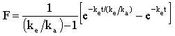
where t = time (min), and k_e and k_a are the first-order elimination and absorption rate constants (min-1), respectively. We'll plot an example time course and fit the curve to the data to obtain an estimate of the rate constants.

Enter the Data

In the Welcome to GraphPad Prism dialog box, select Create an XY data table. Under the X category, select Numbers, and under the Y Columns category, choose Enter and plot a single Y value for each point.

Enter the data as shown below.

For this example, we're assuming that the Y values do not require correction by subtraction of a baseline-the minimum Y value is already 0. If you wish to subtract a baseline value from each Y value in a data set, Prism can perform automatic baseline corrections.

Click the Graphs section in the Navigator panel to view the graph:

Fit the Curve

With the graph displayed, click on the Analyze button. From the XY analyses category, select Nonlinear regression (curve fit).

In the Parameters: Nonlinear regression dialog box, select New and, from the list, click Create new equation.

The User-defined Equation dialog is displayed. Enter a Name for this curve-fit analysis (which will be added to the menu the next time you view it). Now enter your equation, in single-line form, into the Definition box. You are limited to certain types of equations and must adhere to a few simple syntax rules. 

Thus, you must designate the dependent and independent variables as Y and X, respectively, and you must write the equation so that Y is isolated on the left-hand side. Our equation can be written on a single line as follows:

You can enter comments, to prompt your memory or to help other users understand your equation, by writing lines beginning with a semicolon.

When you're done entering your equation, click the Rules for Initial Values tab. 

Prism reads your equation and, after eliminating X, Y, and operators, arrives at the "parameters" to be fit, in this case, K_e and K_a. Curve fitting is an iterative, trial-and-error process of substituting values for the parameters in your equation in order to maximize the goodness of fit between your experimental data and the resulting substituted equation. Prism therefore must have an initial "guess" for the value of each parameter, that is, it must have a starting point for the process. When you use one of the built-in equations, Prism derives its own initial values, choosing numbers that are related to your experimental data by programmed "rules". For User-defined equations, Prism has no such rules, so you must provide either those rules or explicit initial values.

In the Rules for Initial Values dialog box, an explanatory note prompts you to enter a number into the first column and the relational rule, or "multiplier" into the second column.

Click OK to fit the curve. The Results sheet appears, this time showing the fitted values for K_e and K_a.

Click the Graphs section to view the graph with curve automatically added on top.

¹ Neubig, R. R., The Time Course of Drug Action, in Principles of Drug Action (W.B. Pratt and P. Taylor, eds.), 3rd Edition, Churchill Livingtone Inc., 1990.