Introduction

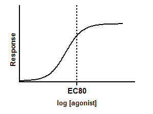
Many log(dose) response curves follow the familiar symmetrical sigmoidal shape. The usual goal is to determine the EC50 of the agonist - the concentration that provokes a response half way between the basal (Bottom) response and the maximal (Top) response. But you can determine any spot along the curve, say a EC80 or EC90.

Many dose-response curves have a standard slope of 1.0. This model does not assume a standard slope but rather fits the Hill Slope from the data. Hence the name Variable slope model. This is preferable when you have plenty of data points.

Step by step

Create an XY data table. Enter the logarithm of the concentration of the agonist into X. Enter response into Y in any convenient units. Enter one data set into column A, and use columns B, C... for different treatments, if needed.

From the data table, click Analyze, choose nonlinear regression, and choose the panel of equations:  Dose-Response -- Special. Then choose "log(Agonist) vs. response -- Find ECanything".

You must constrain the parameter F to have a constant value between 0 and 100. Set F to 80 if you want to fit the EC80. If you constrain F to equal 50, then this equation is the same as a variable slope dose-response curve.

Consider constraining the parameter HillSlope to its standard value of 1.0 of -1. This is especially useful if you don't have many data points, and therefore cannot fit the slope very well.

If you have subtracted off any basal response, consider constraining Bottom to a constant value of 0.

Model

logEC50=logECF - (1/HillSlope)*log(F/(100-F))

Y=Bottom + (Top-Bottom)/(1+10^((LogEC50-X)*HillSlope))

Interpret the parameters

ECf is the concentration of agonist that gives a response F percent of the way between Bottom and Top. Prism reports both the ECF and its log.

HillSlope describes the steepness of the family of curves. A HillSlope of 1.0 is standard, and you should consider constraining the Hill Slope to a constant value of 1.0. A Hill slope greater than 1.0 is steeper, and a Hill slope less than 1.0 is shallower.

Top and Bottom are plateaus in the units of the Y axis.

Adapting this equation

ICanything

This equation can also fit inhibitory data where the curve goes downhill rather than uphill. The best-fit value of the Hill Slope will be negative in this case.The result will always be reported as ECf. Let's say you set F=80. Then the ECf for inhibitory data would be the concentration (X value) required to bring the curve down to 80%. If you want the concentration that brings the curve down by 80%, to 20%, then you'd need to set F equal to 20. If you want the result to say "ICF" rather than "ECF", clone the equation and then edit to make that change

X is concentration rather than log concentration

The dose response equations where X is dose or concentration (rather than its logarithm) can be easily adapted to fit the ECF or ICF. Simply clone the equation and add one line to the top that turns EC50 into an intermediate variable and adds the parameters ECF (which you'll fit) and F (which you'll set as a constant). For example the [Agonist] vs. response -- variable slope equation becomes:

EC50 = ECF/((F/(100-F))^(1/HillSlope))

Y=Bottom + (X^Hillslope)*(Top-Bottom)/(X^HillSlope + EC50^HillSlope)