This guide will walk you through the process of performing multiple logistic regression with Prism. Logistic regression was added with Prism 8.3.0
The data
To begin, we'll want to create a new Multiple variables data table from the Welcome dialog
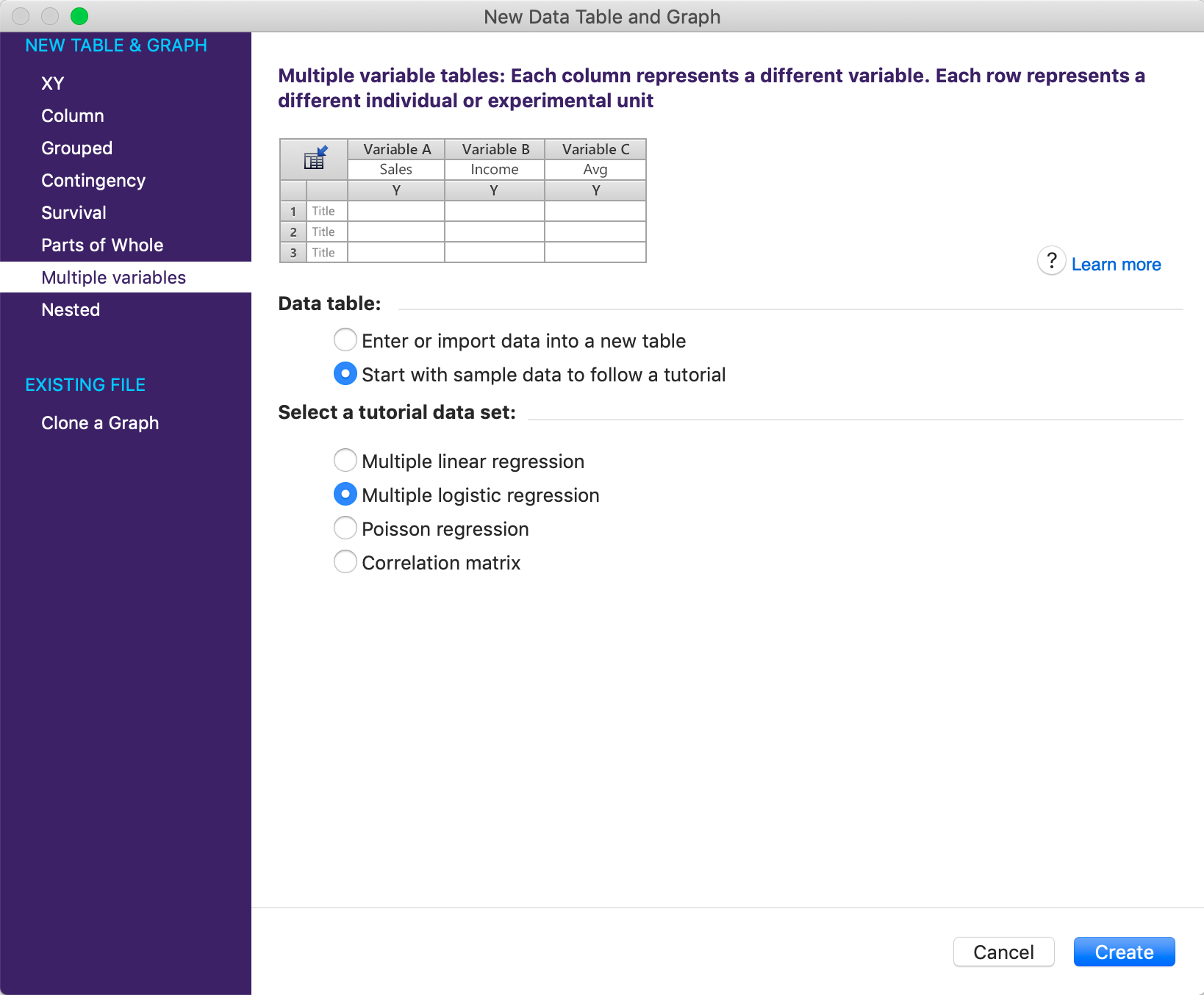
Choose the Multiple logistic regression sample data found in the list of tutorial data sets for the multiple variables data table.
The sample data has five total columns: "Survived?", "Age (in years)", "Male?", "1st Class?", and "2nd Class?".
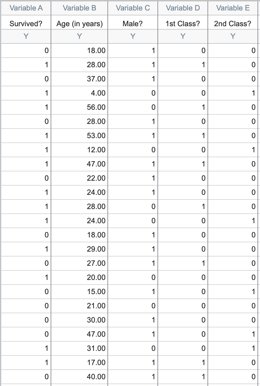
These data represent 1,314 passengers on board the RMS Titanic, with each row representing a different passenger (note that the crew is not included in this data set, and that the official number of passengers varies among available sources). The first column "Survived?" provides the fate for each passenger, with a 1 indicating that the passenger survived and a 0 indicating that the passenger died when the ship sank. The other four columns provide demographic information and the ticketed cabin for each passenger. Note that three of these four columns are also coded (with all values in these columns being either a 1 or 0). A brief explanation of how this coding works is given below. To get straight to the analysis, skip to "Initiating the analysis"
What about 3rd Class? (A quick intro to dummy coding)
As mentioned above, a number of the variables in this data set are coded as either a 1 or 0. In each case, the column titles have been entered as a question, and the presence of a 1 for a given observation means that the answer to the question is "yes", while the presence of a 0 for an observation means that the answer to the question is "no". For example, we can discern some information about the passenger in the first row in the table above. The 0 in the first column means that the passenger did not survive, they were 18 years old, and the 1 in the third column indicates that the passenger was male.
But what ticket class was this passenger? We see in the fourth column that the passenger wasn't 1st class, and we see in the fifth column that the passenger wasn't 2nd class (with 0s in both of these columns). Thus, we can conclude that this passenger must have been 3rd class (because he wasn't 1st or 2nd class, and those are the only possibilities).
When a variable is categorical (survived/died, male/female, 1st/2nd/3rd class, etc.), we can encode those responses as a set of 0s and 1s in a process called dummy coding (there are other coding techniques, but dummy coding is probably the easiest to understand). Using dummy coding, variables with two outcomes (survived/died, male/female, etc.) end up getting coded using one column. You don't need one column for "Male?" and one column for "Female?" because you can get all of the information from a single column. Similarly, variables with three outcomes (first class/second class/third class) end up getting coded using two columns. In this case, we don't need a column for "3rd Class?" because we can discern that information from the values in the other two columns. In fact, if you DID try to include a column for "3rd Class" in the logistic regression model, the analysis would fail because of linear dependence of the variables.
Initiating the analysis
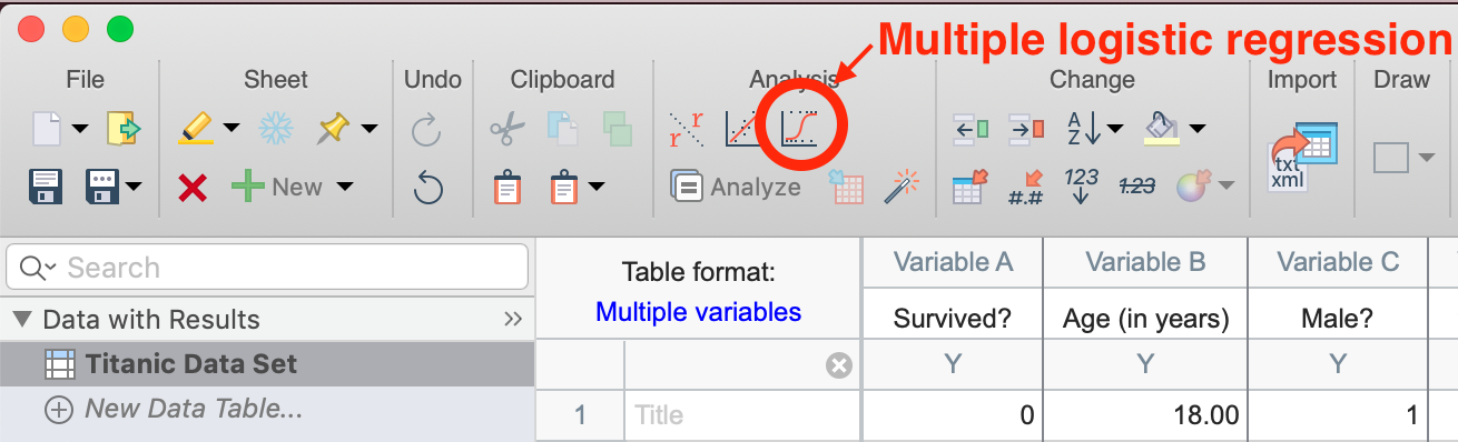
Click on the multiple logistic regression button in the toolbar (shown below), or click on the "Analyze" button in the toolbar, and then select "Multiple logistic regression" from the list of available Multiple variable analyses.
The analysis dialog
After clicking the multiple logistic regression button, the parameters dialog for this analysis will appear. For the purposes of this walkthrough, we'll simply accept most of the default options. The results for these default options are discussed below, but there are many more options available on each of the tabs of the multiple logistic regression parameters dialog. Something that we will change to make interpretation of the results a bit easier are the labels for the "Negative" and "Positive" outcomes (i.e. what it means for the entered response to be a 0 or a 1). In the space for the "Negative Outcome" label, enter "Died", and in the space for the "Positive Outcome" label, enter "Survived".

Once you click "OK", you'll be taken to the main results sheet which will be discussed in the next section.
Results of logistic regression
Parameter estimates
The first thing that you'll see on the results sheet are the best fit value estimates along with standard errors and 95% confidence intervals for β0 along with one parameter estimate for each component (main effect or interaction) in the model. In this case, we have the parameter estimate for the intercept (β0) and four main effects.
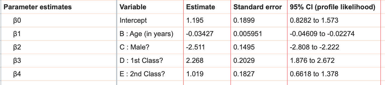
Interpretation of these parameters is a little different than with linear regression due to the fact that logistic regression models the log odds. Make sure you understand the relationship between log odds, odds, and probability before trying to make sense of these parameter estimates. In this example, we see that the estimate for "Male?" is -2.511, while the estimate for "1st class?" is 2.268. This means that if a passenger was male (all other variables held constant), their log odds of survival was decreased by 2.511, while if a passenger was in first class (all other variables held constant), their log odds of survival was increased by 2.268.
Odds ratios
As an alternative to seeing the results as log odds, Prism also reports the odds ratios and their 95% confidence intervals (reported farther down on the results sheet).
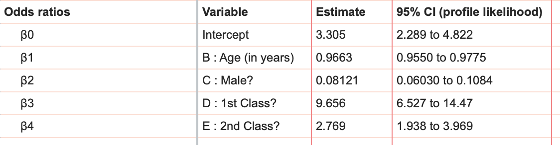
A more detailed explanation of odds ratios can be found here, but what the odds ratios for each variable (β1, β2, β3, and β4) tells us is that increasing that variable by 1 multiplies the odds of success by the value of the odds ratio. The odds ratio for "Age (in years)" is reported as 0.9663. This means that for each year older a passenger was, their odds of survival was multiplied by 0.9663. Since this odds ratio is less than 1, this means that as a passengers age increases, their odds of survival actually decreased (all other factors held constant).
Another point to note is that, because we've used dummy coding for some of our variables, these odds ratios assume a certain "default" or "reference" status for these passengers. For example, we can set the variables "Male?", "1st Class?", and "2nd Class?" to equal zero to investigate the effects of age on the odds of survival. However, because we've used dummy coding, what we're actually looking at is the effect of age on the odds of survival for 3rd class female passengers. Let's say we determined the odds of survival for a 3rd class female passenger at 25 years of age. In this case, the values of "Male?", "1st Class?", and "2nd Class?" would all be 0, and the resulting Odds would be 1.402. Knowing this, we could then quickly determine the odds of survival for a 1st class female passenger at age 25 (Odds = 1.402*9.656 = 13.538). Thus, when using dummy coding, the odds ratio actually tells us how the odds change relative to the reference case.
Review of probability and odds
In case you haven't read about the relationship of probability and odds, here's a quick summary:
Odds = Probability of success/Probability of failure
Since the probability of failure is just 1 - Probability of success, we can write this as:
Odds = (Probability of success)/(1 - Probability of success)
For example, let's say there's a 75% probability of success, the odds would then be calculated as:
Odds = 0.75/(1 - 0.75) = 0.75/0.25 = 3
Commonly, we would say that "the odds are 3:1" (read "three to one").
P values
By default, P values for the parameter estimates aren't given in the results, and thus won't be discussed here. However, you can select to display these values using the Options tab of the Multiple Logistic Regression Parameters dialog. You'll also want to read about how to interpret these values if you choose to have Prism report them.
Model diagnostics
The next section of the multiple logistic regression results provides a number of useful model diagnostics for determining how well the data fit the selected model. By default, the two values reported here include the degrees of freedom and corrected Akaike's Information Criterion (AICc) for both an "Intercept-only model" and the "Selected model". These two models are fairly easy to describe:
•Intercept-only model: a logistic regression model including only the intercept term β0. This model uses none of the independent variables when predicting the outcome. Therefore the same prediction is made for every case.
•Selected model: the logistic regression model that you chose to fit to the data
The results of this section actually provide you with a way to determine if your selected model does a better job at fitting the data than an intercept-only model. Another way to say this is that the variables in your selected model provide useful information about the observed data. The way you determine which model does a better job fitting the data is by using the AICc. The way the AICc is calculated is a bit complex, but interpretation in this case is fairly simple: a smaller AICc indicates a better model fit. With values of 1746 for the intercept-only model and 1235 for our selected model, we can determine that our selected model does a better job describing the observed data.
Row prediction
The next section that we'll discuss is actually not on the main results tab. At the top of the main results sheet, you'll see a tab titled "Row Prediction". When clicking on this tab, Prism will provide a complete list of predicted probabilities for all observations with complete information for each variable:

This table provides predicted probabilities for all complete observations in the table. This includes both observations from the data that were fit as well as observations that were entered without a Y value. In this example, we could imagine a hypothetical passenger who was a male, age 34, with a second class ticket. Surprisingly, no such passenger exists in the current data set. However, we could enter the corresponding values for this hypothetical passenger into the original table on row 1315 for the corresponding variables, leaving the cell for "Survived?" blank. Since the survival cell is blank, adding this row to the table won't affect most of the results of logistic regression. but Prism will show you the predicted probability of this hypothetical individual surviving.
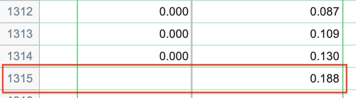
This result tells us that - based on the observations of the other 1314 passengers - our new hypothetical passenger (34 year old male with 2nd class ticket) would have only an 18.8% probability of surviving!
The ROC curve and the area under the ROC curve
Going back to the "Tabular results" section of the results sheet, the next section of the results deals exclusively with something called an ROC curve. The ROC curve for this analysis is provided in the Graphs section of the Navigator, and looks like this:

Understanding ROC curves takes a bit of experience, but ultimately what these graphs are showing you is the relationship between the model's ability to correctly classify successes correctly and its ability to classify failures correctly. The way the model classifies observations is by setting a cutoff value. Any predicted probability greater than this cutoff is classified as a 1, while any predicted probability less than this cutoff is classified as a 0. If you set a very low cutoff, you would almost certainly classify all of your observed successes correctly. The proportion of observed successes correctly classified is referred to as the Sensitivity, and is plotted on the Y axis of the ROC curve (a Y value of 1 represents perfect classification of successes, while a Y value of 0 represents complete mis-classification of successes).
However, with a very low cutoff, you would also likely incorrectly classify many failures as successes as well. Specificity is the proportion of correctly classified failures, and "1-Specificity" is plotted on the X axis (so that an X value of 0 represents perfect classification of failures, and an X value of 1 represents complete mis-classification of failures).
You can imagine that as the cutoff is varied (from 0 to 1), there will be a trade-off of the observed successes and failures that are correctly (and incorrectly) classified. That trade-off is what the ROC curve shows: as sensitivity increases, specificity must decrease (i.e. 1-specificity must increase). Each point along this ROC curve represents a different cutoff value with corresponding sensitivity and specificity values.
The area under the ROC curve (AUC) is a measure of how well the fit model correctly classifies successes/failures. This value will always be between 0 and 1, with a larger area representing a model with better classification potential. In our case, the AUC for the the ROC curve (depicted below) is 0.8889, and is listed in the results table along with the standard error of the AUC, the 95% confidence interval, and P value (null hypothesis: the AUC is 0.5). Read more about ROC curves for logistic regression for even more information and some of the math involved.


Classification table
As discussed in the previous section, the area under the ROC curve considers every possible cutoff value for distinguishing if an observation is predicted to be a "success" or a "failure" (i.e. predicted to be a 1 or a 0). In this section of the results, a single cutoff value is used to generate a table of results that provide the number of observed 1s and 0s along with the predicted number of 1s and 0s. The default cutoff value used to generate this table is 0.5, but this can be changed manually in on the "Goodness-of-fit" tab of the multiple logistic regression parameters dialog.
Below is the table containing our results for a cutoff of 0.5:
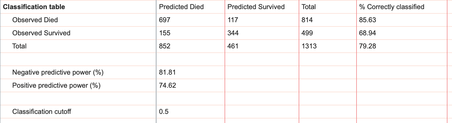
From this table, you can quickly see the total number of observed died (814), total number of observed survived (499), the predicted total number of died (852), and the predicted total number of survived (461). Additionally, this table provides the breakdown for how model predicted each of the the observed survived and died, along with the percent of observed survived and died that were classified correctly.
Finally, the classification table provides information on the negative and positive predictive power, which are other ways that the performance of a model can be assessed.
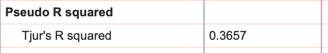
Pseudo R squared
Another way to quantify how well a logistic regression model fits to the given data is by using metrics known as pseudo R squared values. It's important to note right away that although "R squared" may be in their name, these metrics simply cannot be interpreted in the same way that R squared for linear and nonlinear regression is interpreted. Instead, these values provide different kinds of information about the model fit, and will take on values between 0 and 1, with higher values indicating a better fit of the model to the data.
Of the various pseudo R squared values that Prism can calculate, Tjur's R squared is arguably the easiest to interpret, and is the only one reported by default. To calculate Tjur's R squared, find the average predicted probability of success for the observed successes and the average predicted probability for the observed failures. Then calculate the absolute value of the difference between these two values. That's Tjur's R squared! Values close to 1 would indicate that there is a clear separation between observed 0s and observed 1s, while a a Tjur's R squared close to zero would indicate that the average predicted probability of success for both groups were almost the same (i.e. the model didn't do a good job separating the observed 0s and 1s).
Predicted vs Observed graph
Another way to visually inspect how well the selected model does at predicting successes and failures is to look at the Predicted vs Observed graph provided in the Graphs section of the Navigator by default. The graph for our data looks like this:

Interpretation of this graph is fairly straightforward. In this graph, we can see that there are two groups (one for the group of individuals that survived and one for the group of individuals that did not). We can also see the distribution of predicted probabilities for both of those groups. Looking at the violin plot for the group of individuals that died, we can see that the majority of them had predicted probabilities of survival well below 0.5 (with a median of 0.1383 and mean of 0.2411). We can also see that the model did not perform as well with classifying the group of observed survivors. For this group, we see that the predicted probabilities are more uniformly distributed (with a median of 0.6564 and a mean of 0.6068). Of course, the predictions are based only on the independent variables (age, gender and class of service) and ignore the actual outcome.
Hypothesis tests
If we click back to the "Tabular results" tab of the results sheet, we can continue investigating the other results reported by multiple logistic regression. By default, the next section of the results provides one of two ways that Prism can test how well the model fits the data. This test is known as the Hosmer-Lemeshow test, and tests the null hypothesis that the selected model is correct. The specifics of this test are a bit complicated, but based on our data, we would likely elect to reject this null hypothesis that the specified model is correct.

Given this result, we may choose to investigate additional factors that could have influenced the probability of survival that weren't included in our original model. However, it's very important to note that the Hosmer-Lemeshow test has been shown to be sensitive to slight changes in its calculation method, and as such is included in Prism's results primarily as a means to validate findings in Prism with other software applications.
A small P value does NOT necessarily mean that your model is somehow inherently "bad". After all,
"All models are wrong, but some are useful..."
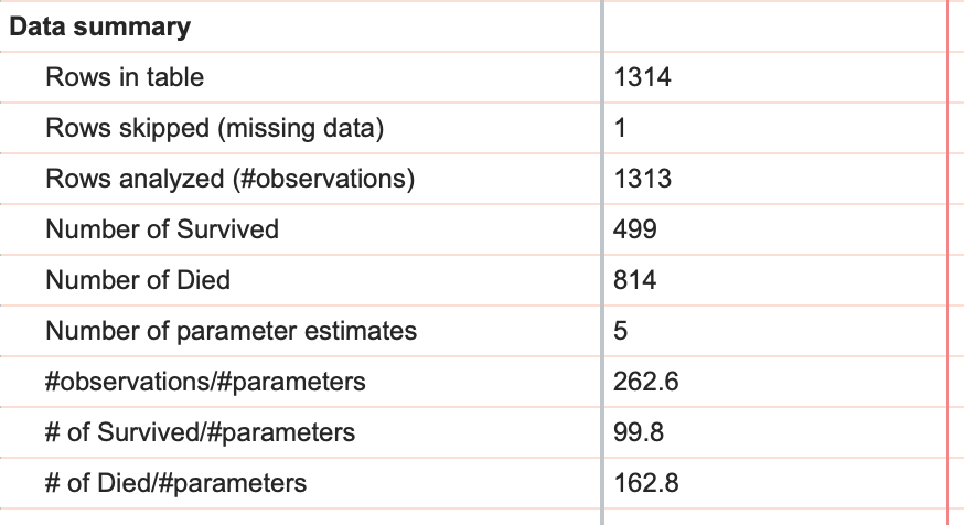
Data Summary
The final pieces of information that Prism provides from multiple logistic regression are given in the form of a data summary that includes the number of rows in the data table, the number of rows that were skipped, and the difference of these two values providing the number of observations in the analysis. Note that in our data set, we have 1314 rows in the table (1315 if you added the example for interpolation), but only 1313 rows analyzed. This difference is due to the fact that the outcome (survived or didn't) was unknown for one (or more) passengers, and so these rows were skipped when fitting the model.
Additionally in the data summary, the total number of 1s and the total number of 0s is given as "Number of Survived" and "Number of Died". Finally, three ratios are provided: number of observations to number of parameters, number of survived to number of parameters, and number of died to number of parameters (we recommend that these last two ratios should be at least 10 for logistic regression).