This guide will walk you through the process of performing simple logistic regression with Prism. Logistic regression was added with Prism 8.3.0
The data
To begin, we'll want to create a new XY data table from the Welcome dialog
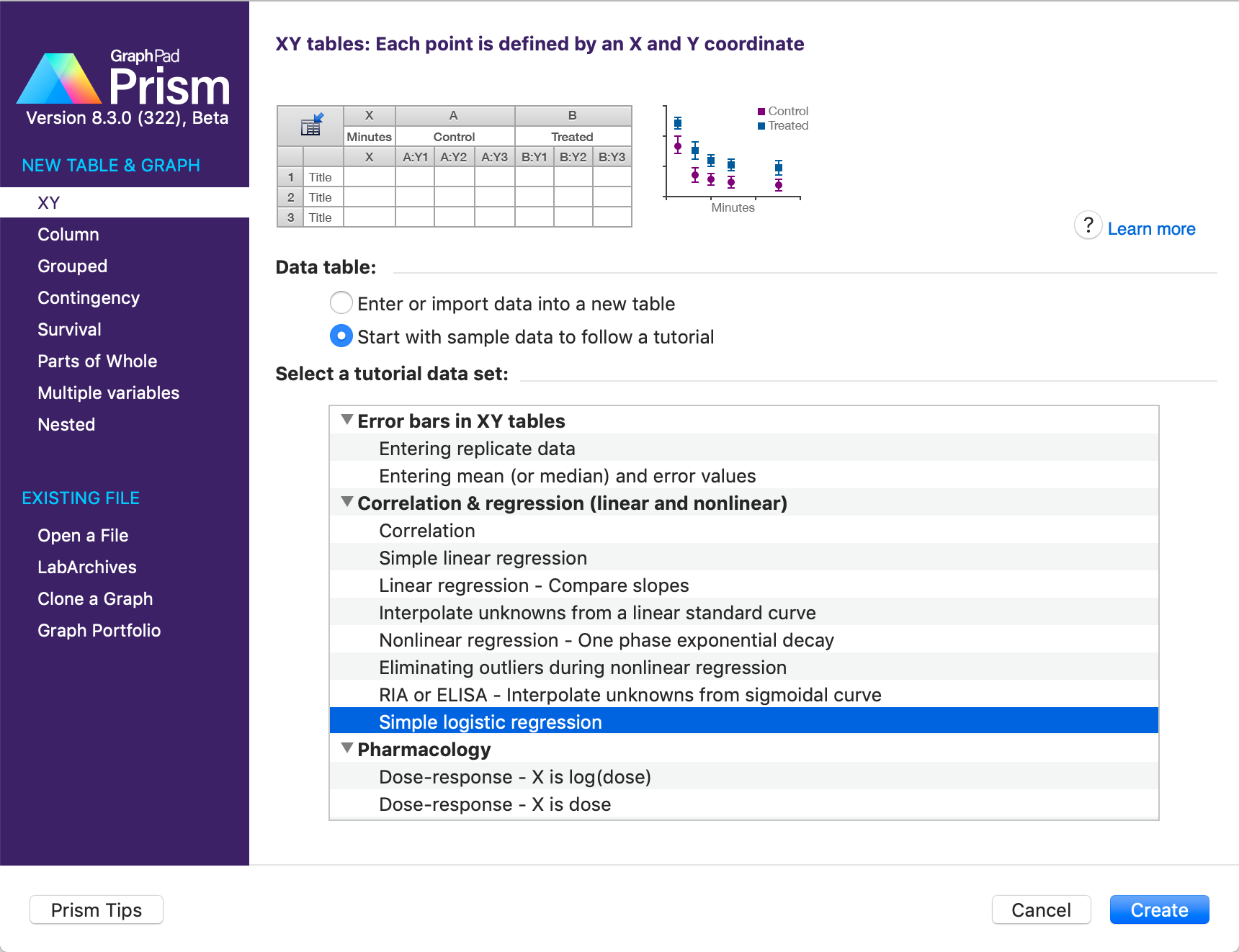
For the purposes of this walkthrough, we will be using the Simple logistic regression sample data found in the "Correlation & regression" section of the sample files. To use this data, click on "Simple logistic regression" in the list, and then click "Create". You will then be shown a set of data with two columns: "Hours Studied" in the X column and "Test Passed?" in the Y column.
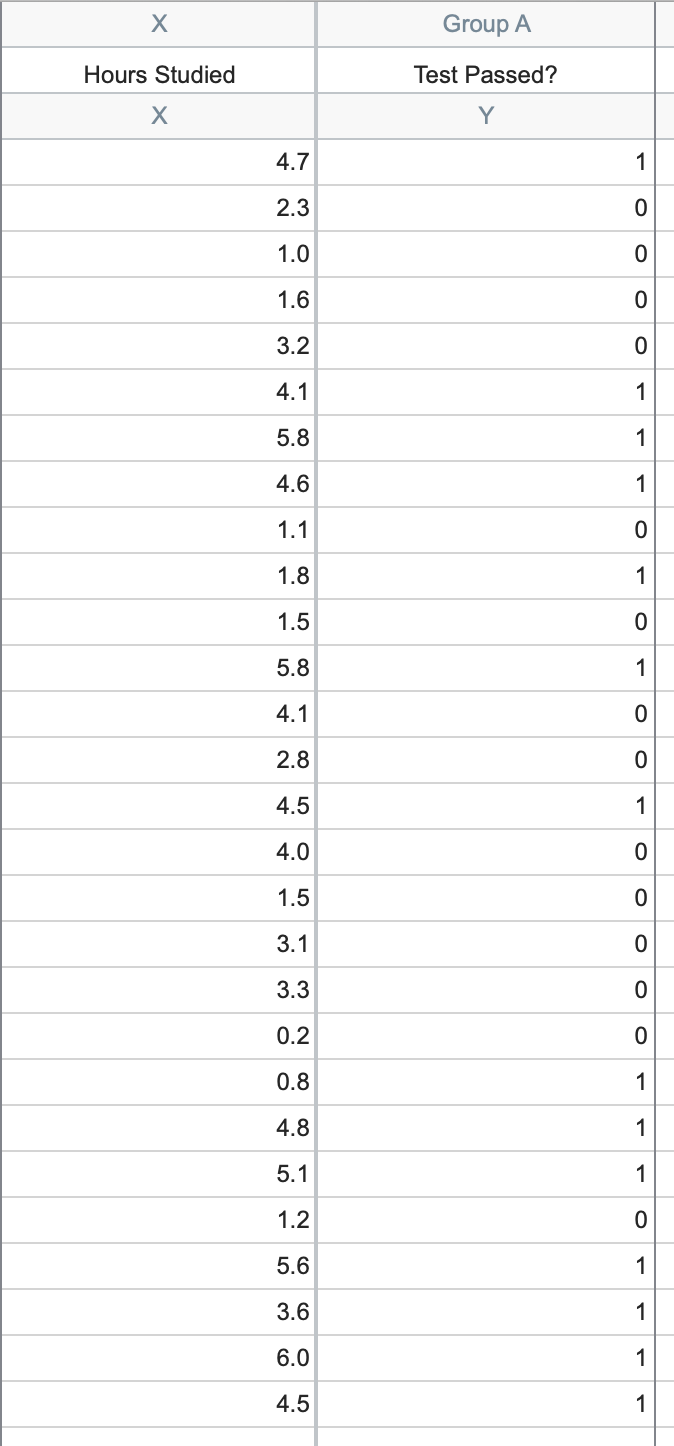
This data represents a collection of 125 students and the amount of time that they spent preparing for a test along with the outcome of the test: did the student pass (entered as a 1 in the data table) or did the student fail (entered as a 0 in the data table)?
Initiating the analysis
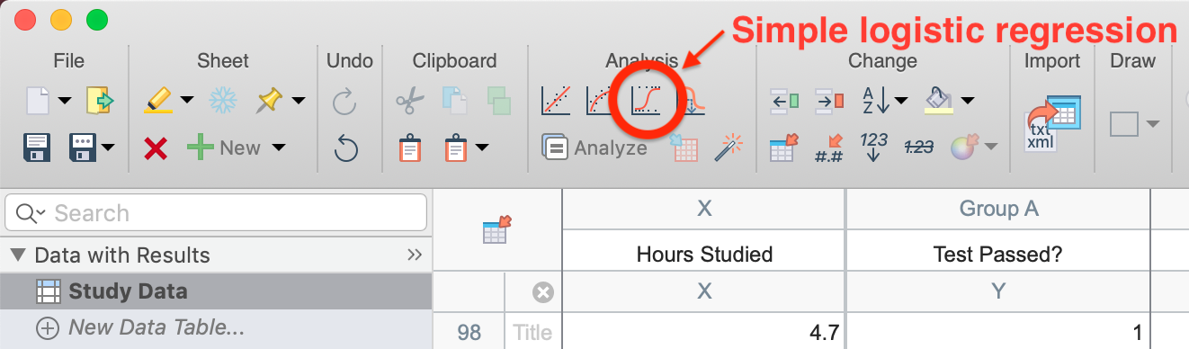
To perform simple logistic regression on this dataset, click on the simple logistic regression button in the toolbar (shown below). Alternatively, you can click on the "Analyze" button in the toolbar, then select "Simple logistic regression" from the list of available XY analyses.
The analysis dialog
After clicking the simple logistic regression button, the parameters dialog for this analysis will appear. For the purposes of this walkthrough, we won't need to change any of the default options. The results for some of these options are discussed below, but additional information can for these options can be found here.
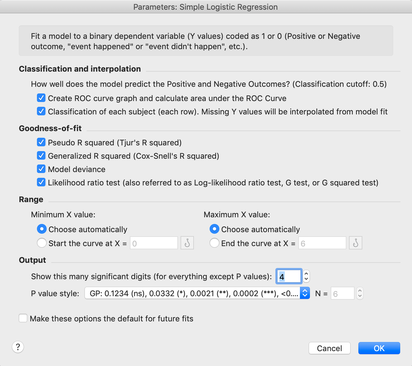
Once you click "OK", you'll be taken to the main results sheet which will be discussed in the next section.
Results of simple logistic regression
Parameter estimates
The first thing that you'll see on the results sheet are the best fit value estimates along with standard errors and 95% confidence intervals for both β0 and β1.
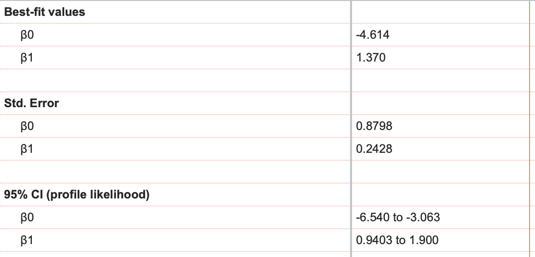
These parameters are sometimes referred to as the "intercept" and "slope", respectively, based on their relationship to the "log odds".
Odds ratios
Because it is hard to directly interpret β0 and β1, it's common to look instead to the odds ratios and their 95% confidence intervals (reported farther down on the results sheet).
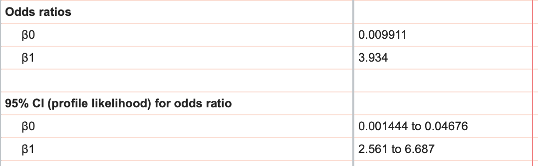
A more detailed explanation of odds ratios can be found here, but what the odds ratio for β1 tells us is that increasing X by 1 multiplies the odds of success by the value for β1. Take the values in these results, for example. Recall that X represents the number of hours studied. Thus, an odds ratio of 3.934 tells us that for every additional hour studied, the odds of passing the test are multiplied by almost 4!
In case you haven't read about the relationship of probability and odds, here's a quick summary:
Odds = Probability of success/Probability of failure
Since the probability of failure is just 1 - Probability of success, we can write this as:
Odds = (Probability of success)/(1 - Probability of success)
For example, let's say there's a 75% probability of success, the odds would then be calculated as:
Odds = 0.75/(1 - 0.75) = 0.75/0.25 = 3
Commonly, we would say that "the odds are 3:1" (read "three to one").
X at 50%
Another key value that Prism reports for simple logistic regression is the value of X when the probability of success is predicted to be 50% (or 0.5). Interestingly, using our equation for odds given above, we can see that when probability is 50%, the odds are equal to 1 (also known as "even odds"). In our case, the value of X at 50% is 3.37, meaning that for those students that studied 3.37 hours, the odds of passing the test were 1:1 (a 50% probability of passing.. not great!).
If we combine this result with the odds ratio, we can quickly determine the odds and probability of passing if the student studies one hour more. Remember, the odds ratio that Prism reports tells us by how much the odds are multiplied when X increases by 1. We know that the odds are 1 when X is 3.37, and the odds ratio is 3.934. Thus, increasing X by 1, from 3.37 to 4.37 gives us a new odds of 1*3.934, or just 3.934. That is the predicted odds of passing for students that studied 4.37 hours (just one hour extra).
It is easy to convert this odds to a probability:
Odds = 3.934 = (Probability of success)/(1 - Probability of success)
3.934*(1 - Probability of success) = Probability of success
3.934 - 3.934*(Probability of success) = Probability of success
3.934 = Probability of success + 3.934*(Probability of success)
3.934 = (Probability of success)*(1 + 3.934)
3.934 = (Probability of success)*4.934
Probability of success = 3.934/4.934
Probability of success = 0.797 or 79.7%
The logistic regression curve
If we break away from the results sheet for just a moment, we can take a look at the curve that logistic regression plotted for our data. This graph (shown below), confirms some of the observations that we made in the previous sections:

The curve on this graph plots the predicted probability of passing the test (Y) as a function of the number of hours studied (X). As we discussed, we can quickly see that for a study time of 3.37 hours, the predicted probability of passing the test is 50%:

We can also confirm our claims about odds ratios from this graph. We can see that by increasing the amount of time studied by one hour (to 4.37 hours total), the predicted probability of passing the test increases to ~80%:

In fact, you can use this curve to determine the predicted probability of passing the test for any given amount of time studied. The next section discusses how to determine the predicted probability for any entered X value
Row prediction
If we switch back to the main results sheet for simple logistic regression, you'll see at the top a sheet tab titled "Row prediction". When clicking on this tab, Prism will provide a complete list of predicted probabilities for all entered X values:
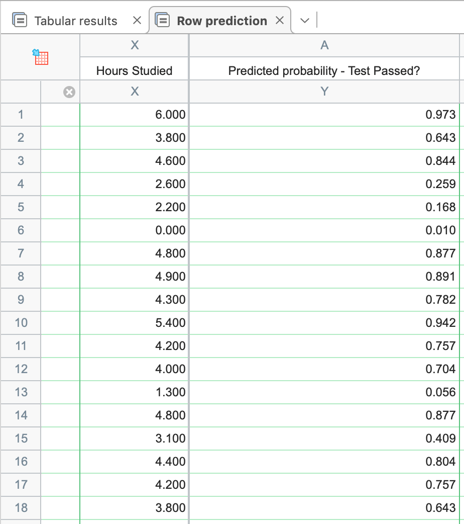
This table provides predicted probabilities for all X values in the data table. This includes both X values from the data that were fit as well as lone X values that were entered without a Y value. Say, for example, you wanted to know the probability of passing the test given this model and a study time of 5.7 hours. Of the 125 students in this data set, none studied 5.7 hours, but going back to the original data table, you can enter 5.7 at the bottom of the X column (without an associated Y value), and then return to the Row Classification table:
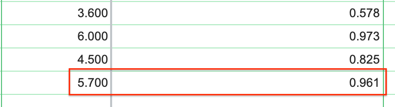
This result tells us that - based on the observations of the 125 students - if a new student were to study for this same test for 5.7 hours, they would have a 96.1% probability of passing!
Hypothesis tests
If we click back to the "Tabular results" tab of the results sheet, we can continue investigating the other results reported by simple logistic regression. The next section of the results provides two different ways to test how well the model fits the data. While these tests are quite similar, it's important to understand how each of them work and the hypothesis that each are testing to interpret the results.
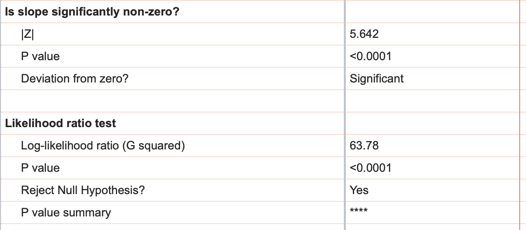
Based on the results given for our data, we can conclude that the effect of studying (given by the coefficient β1) is definitely non-zero; in other words, the amount of time studied had a definite effect on the probability of passing the test.
The ROC curve and the area under the ROC curve
The next section of the results deals exclusively with something called an ROC curve. The ROC curve for this analysis is provided in the Graphs section of the Navigator, and looks like this:

Understanding ROC curves takes a bit of experience, but ultimately what these graphs are showing you is the relationship between the model's ability to correctly classify successes correctly and its ability to classify failures correctly. The way the model classifies observations is by setting a cutoff value. Any predicted probability greater than this cutoff is classified as a 1, while any predicted probability less than this cutoff is classified as a 0. If you set a very low cutoff, you would almost certainly classify all of your observed successes correctly. The proportion of observed successes correctly classified is referred to as the Sensitivity, and is plotted on the Y axis of the ROC curve (a Y value of 1 represents perfect classification of successes, while a Y value of 0 represents complete mis-classification of successes).
However, with a very low cutoff, you would also likely incorrectly classify many failures as successes as well. Specificity is the proportion of correctly classified failures, and "1-Specificity" is plotted on the X axis (so that an X value of 0 represents perfect classification of failures, and an X value of 1 represents complete mis-classification of failures).
You can imagine that as the cutoff is varied (from 0 to 1), there will be a trade-off of the observed successes and failures that are correctly (and incorrectly) classified. That trade-off is what the ROC curve shows: as sensitivity increases, specificity must decrease (i.e. 1-specificity must increase). Each point along this ROC curve represents a different cutoff value with corresponding sensitivity and specificity values.
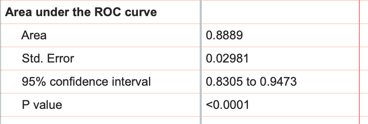
The area under the ROC curve (AUC) is a measure of how well the fit model correctly classifies successes/failures. This value will always be between 0 and 1, with a larger area representing a model with better classification potential. In our case, the AUC for the the ROC curve (depicted below) is 0.8889, and is listed in the results table along with the standard error of the AUC, the 95% confidence interval, and P value (null hypothesis: the AUC is 0.5). Read more about ROC curves for logistic regression for even more information and some of the math involved.

Goodness of fit and additional model details
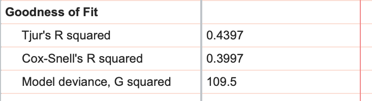
In the final section of calculated results, Prism provides some additional metrics that attempt to summarize how well the model fits the given data. The first two of these are Tjur's R squared and Cox-Snell's R squared, and while "R squared" may be in their name, these metrics simply cannot be interpreted in the same way that R squared for linear and nonlinear regression is interpreted. Instead, these values are known as pseudo R squared values, provide different kinds of information about the model fit. For these metrics, the calculated value will be between 0 and 1, with higher values indicating a better fit of the model to the data.
Of the two pseudo R squared values provided, Tjur's R squared is much easier to calculate and interpret: find the average predicted probability of success for the observed successes and the average predicted probability for the observed failures. Then calculate the absolute value of the difference between these two values. That's Tjur's R squared!
The last metric Prism reports is the model deviance. This value requires by far one of the hardest calculations of the metrics that simple logistic regression reports, and so it won't be explained here. However, this metric provides a numeric estimate for "how likely" it is that the model (with the parameters given earlier in the results) would have generated the observed data. Sounds confusing, but the key here is that if you're comparing multiple models to describe the same data, a smaller value for model deviance represents a better model fit (model deviance cannot be a negative value, with a deviance of zero indicating a perfect fit of the model to the data).
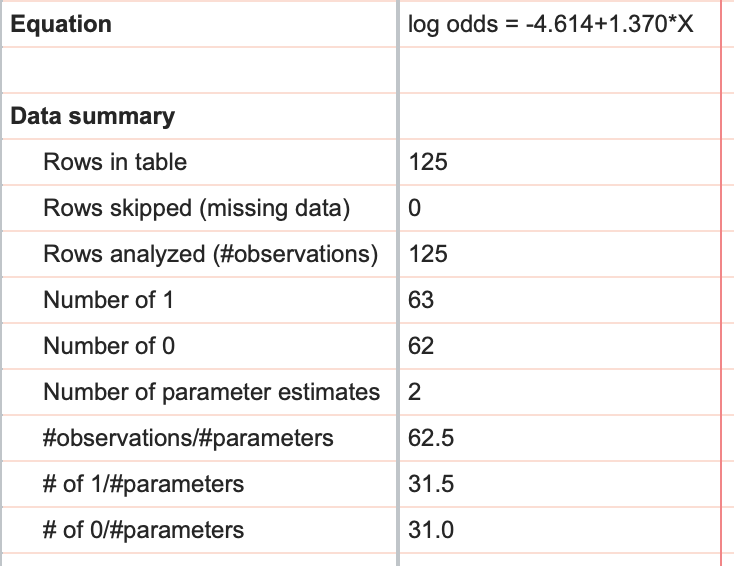
Equation and Data Summary
The final pieces of information that Prism provides from simple logistic regression include the model equation (given in terms of log odds), and a data summary that includes the number of rows in the data table, the number of rows that were skipped, and the difference of these two values providing the number of observations in the analysis. Additionally in the data summary, the total number of 1s and the total number of 0s is given. Finally, three ratios are provided: number of observations to number of parameters, number of 1s to number of parameters, and number of 0s to number of parameters (we recommend that these last two ratios should be at least 10 for logistic regression).