Two ways to perform Kaplan-Meier survival analysis
Prism offers two different ways to perform Kaplan-Meier survival analysis, depending on how your data are structured:
1.Survival data table: This is the traditional approach where time-to-event data and censoring information are entered directly into a specialized survival table format. This method is described in detail on this page.
2.Multiple Variables data table: This approach allows you to perform survival analysis from a Multiple Variables table, which can be more convenient when integrating survival data with other types of data or when importing data from other sources. For information about data structure requirements and how to set up survival analysis from a Multiple Variables table, see Survival analysis from Multiple Variables tables.
Both methods produce identical statistical results. The primary difference is in how the data are structured and a few minor variations in the analysis parameters dialog, as described below.
Prism analyzes data in Survival data tables automatically (no need to initiate an analysis manually)
The survival analysis is unique among the analyses that Prism offers. When data are entered into a survival data table, Prism automatically performs the analysis of the data and generates Kaplan-Meier survival curves. You don’t need to start an analysis using the Analyze toolbar button or selecting the analysis from the Analyze menu, and you don’t need to specify any options on the analysis parameters dialog. Prism will use the default options for the analysis and generate the results for you.
To see the options specified for the analysis, you can access the analysis parameters dialog from the survival analysis results sheet. Simply click on the analysis parameters toolbar button to bring up the dialog.
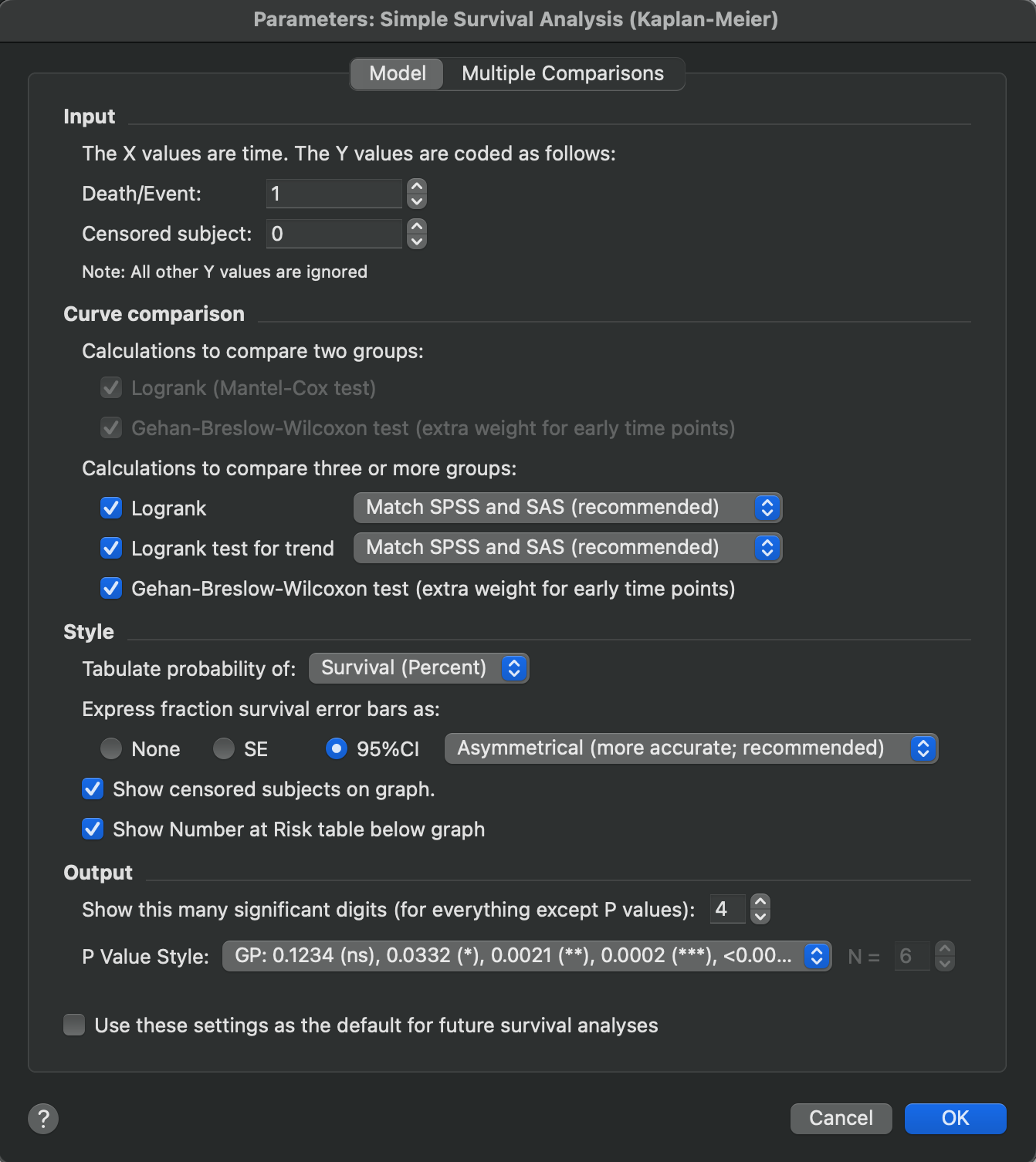
Input
Survival data tables
When performing survival analysis from a Survival data table, you specify numeric codes to indicate censoring and events. The default choices are to use the code "1" to indicate that the event of interest occurred and "0" to indicate that the observation was censored. These codes are nearly universal. However, some institutions use the opposite convention. In Prism, these codes can be specified manually, but they must be integer values.
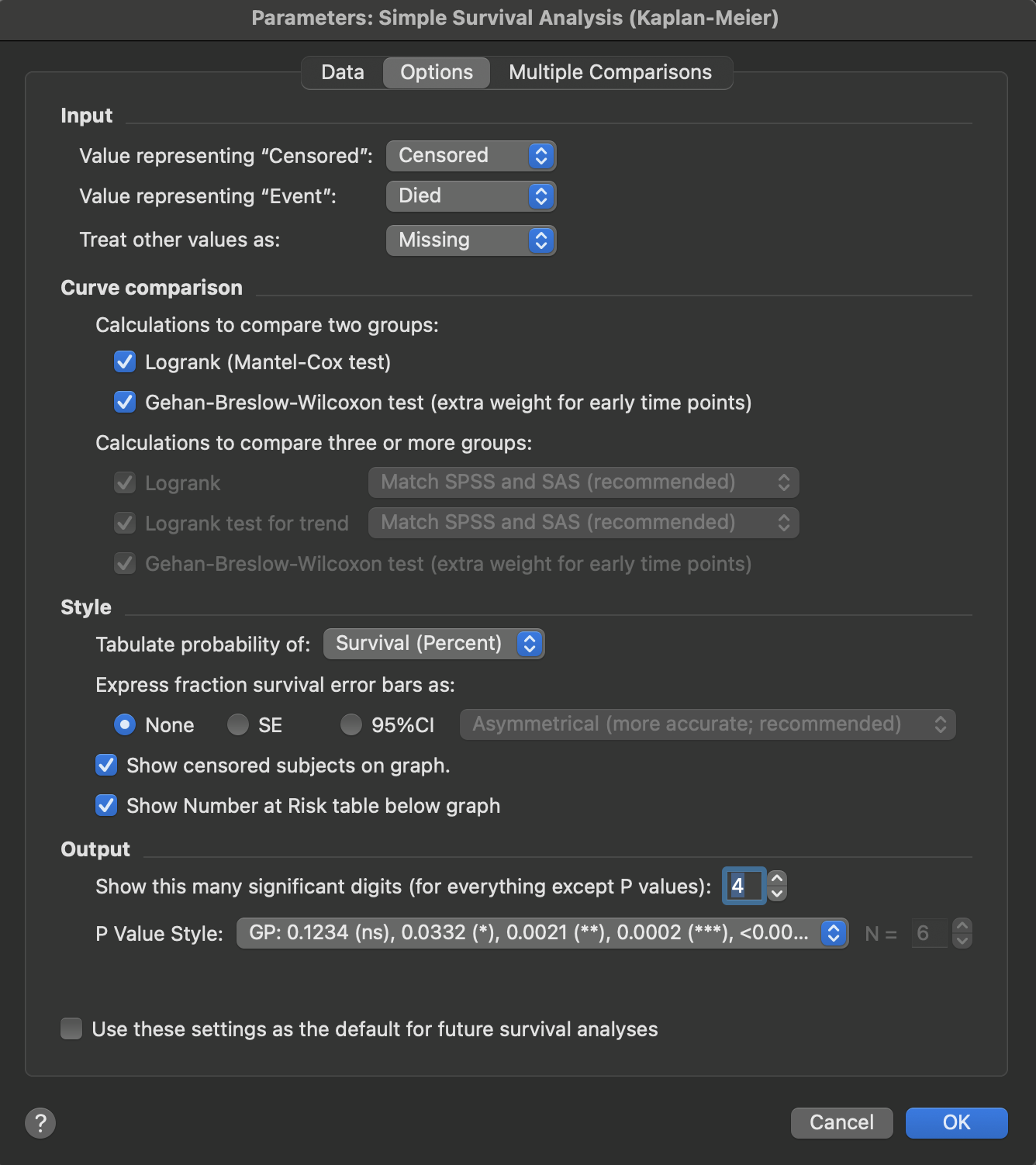
Multiple Variables data tables
When performing survival analysis from a Multiple Variables data table, the Input section works differently. Instead of numeric codes, you specify text values from the variable specified on the Data tab as the grouping variable. These values represent the censored and event categories. This allows you to use descriptive labels (such as "Male" and "Female", or "Died" and "Survived") that may already exist in your data. In case the specified variable contains more than only two levels, you can also specify how to treat other values that don't match either category - typically these are treated as missing data.
Curve comparisons for two survival curves
To compare two survival curves, Prism has two methods available:
•The logrank test. There are two ways to compute this test. The two are almost equivalent, but can differ a bit in how they deal with multiple events occurring at the exact same time (this concept is known as “ties” in the data). Prism uses the Mantel-Haenszel approach, but uses the name ‘logrank’ which is commonly used for both approaches. This method is also known as the Mantel-Cox method.
•The Gehan-Breslow-Wilcoxon test. This method gives more weight to events that occur at early time points, which makes a lot of sense (the earlier an event occurs, the more likely that it’s an important observation since all study participants are expected to experience the event of interest eventually). However, the results of this test can be misleading when a large fraction of the study participants are censored at early time points. In contrast, the logrank test gives equal weight to observations at all time points
The logrank test is more standard. It is the more powerful of the two tests if the assumption of proportional hazards is true. Proportional hazards means that the ratio of hazard functions (deaths per time) is the same at all time points. One example of proportional hazards would be if the control group died at twice the rate as treated group at all time points.
The Gehan-Breslow-Wilcoxon test does not require a consistent hazard ratio, but does require that one group consistently have a higher risk than the other.
If the two survival curves cross, then one group has a higher risk at early time points and the other group has a higher risk at late time points. This could just be a coincidence of random sampling, and the assumption of proportional hazards could still be valid. But if the sample size is large, neither the logrank nor the Wilcoxon-Gehan test rests are helpful when the survival curves cross near the middle of the the time course.
If in doubt, report the logrank test (which is more standard). Choose the Gehan-Breslow-Wilcoxon test only if you have a strong reason to do so.
Curve comparisons for three or more curves
When there are three or more different groups (data sets), Prism provides three methods to compare the resulting survival curves. Details for the logrank test and the Gehan-Breslow-Wilcoxon test are the same as what was provided in the previous section for comparing two survival curves.
•The logrank test. This is the most commonly used test for comparing three or more curves
•The logrank test for trend. This test is only relevant when the order of groups (defined by data set columns in the data table) is logical. Examples would be if the groups are different age groups, different disease severities, or different doses of a drug, each organized in some logical (ascending or descending) order. This left-to-right order of data sets in Prism must correspond to equally spaced ordered categories. If the data sets are not ordered - or are not equally spaced - it makes no sense to choose the logrank test for trend
•The Gehan-Breslow-Wilcoxon test. This method provides more weight to earlier time points. Select this test only if you have a strong reason to do so. Prism computes this test using equation 10.2 from Machin’s text referenced below
With three or more groups, Prism offers a choice of two methods for computing the P value
Match Prism 5 and earlier (conservative, not recommended)
Prism 5 and earlier versions computed a P value to compare three or more groups using a conservative method shown in many textbooks. For each curve, this method computes a chi-square value by comparing the observed and expected number of deaths. It then sums those chi-square values to get an overall chi-square, from which the P value is determined. Here it is as an equation, where Oi is the observed number of deaths in curve i, and Ei is the expected number of deaths:
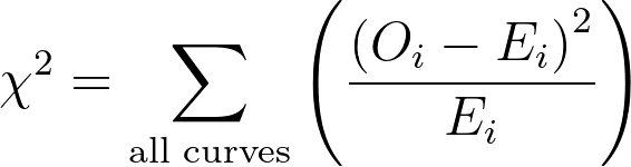
This conservative method is documented in Machin (1), is easy to understand, and works OK. The problem is that the P value is too large (this is what is meant by “conservative”). Choose this method only if you want results to match results from Prism versions 5 and older. Otherwise, choose the recommended method to match SPSS and SAS.
Match SPSS and SAS (recommended)
When comparing three or more groups of survival curves, Prism can also compute P values using a method explained in detail in the manuals of SPSS and NCSS. The method can only be understood in terms of matrix algebra, and the details are beyond the scope of this guide. Like the conservative method, this approach also computes a chi-square statistic. For both methods, the number of degrees of freedom equals the number of groups minus 1. The difference is that the chi-square value for this method is larger than the value generated by the conservative method, and so - subsequently - the P value is smaller.
Style
The way that results are calculated and presented (percents or fractions, death or survival) can also be specified on the Analysis Parameters dialog.
If you choose to plot the 95% confidence intervals, Prism provides two choices. The default is a transformation method, which plots asymmetrical confidence intervals. The alternative is to choose symmetrical Greenwood intervals. The asymmetrical intervals are more valid, and are the recommended option.
The only reason to choose symmetrical intervals is to be consistent with results computed by Prism version 4 and older. Note that “symmetrical intervals won’t always plot symmetrically. The intervals are computed by adding and subtracting a calculated value from the determined percent survival value. At this point, the intervals are always symmetrical, but may go below 0 or above 100 (which doesn’t make any sense in the case of percentages). In these cases, Prism trims the intervals so that the interval cannot extend below 0 or above 100, resulting in an interval that appears asymmetric.
A checkbox allows you to decide whether to plot censored observations or not. The exception is when the largest X value (time) is censored. This is always shown, regardless of whether you choose to display censored values or not.
Finally, a checkbox allows you to indicate if the dynamic number at risk table should be included on the graph of the survival analysis or not.
Output
Choose how many digits of precision to display in the results sheet, and specify the format of calculated P values
Reference
3.David Machin, Yin Bun Cheung, Mahesh Parmar, Survival Analysis: A Practical Approach, 2nd edition, IBSN:0470870400.