The previous pages in this section discuss the Elbow plot and Silhouette score methods of selecting the optimal number of clusters following a clustering analysis. The third method that Prism provides is by using the gap statistic and the resulting gap plot. This is one of the most modern methods commonly used to determine the optimal number of clusters, developed in 2001. This method is also easily the most computationally intensive, and can be a bit confusing to understand. To keep things simple, all you really need to know is that this method determines a “gap statistic” and a standard deviation for each number of clusters into which the data are grouped. Call the gap statistic for “k” clusters “Gap(k)”, and the standard deviation for “k” clusters “sk”. The optimal number of clusters is determined by finding the smallest value of k such that:

Take a look at the gap plot for the same data set that we’ve used in the previous sections exploring the elbow plot and the silhouette plot:

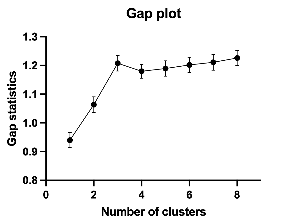
On this graph, you can see that the smallest number of clusters (k) for which the statistic satisfies the definition above is when the number of clusters is three. The gap statistic (plotted on the Y axis) for k=3 is greater than the gap statistic for k=4 minus the standard deviation for k=4, making the optimal number of clusters for this data set three. This is in agreement with both the elbow plot method and the silhouette method.

Prism also provides the option to utilize a set of 17 methods used in Prism's consensus approach for determining optimal cluster numbers, as described on the cluster metrics page.

The remainder of this section is much more math heavy, but will guide you through understanding how the gap statistic is calculated if you’re interested.

A detailed explanation

Like the simple elbow method, the gap statistic method also utilizes a value for the variation or dispersion of data within each cluster. Although there are a variety of different metrics that could be used, the implementation of the gap method in Prism was done such that this measure of dispersion is based off of the WCSS. Recall that the WCSS is a measure of how disperse the data are within the identified clusters. WCSS is determined by calculating the squared distances of each point in a cluster to its assigned cluster center, then summing up all of these squared distances. If the data in the clusters are more spread out (more disperse), then these squared distances will be larger, and the WCSS will be greater. If clusters are more compact, then the WCSS will be smaller.

The primary idea behind the gap statistic method is that if there truly are groups within your data, then clustering your data into these groups will result in clusters that are more compact (less disperse) than performing the same clustering on random data in the same range as your input data. At this point, it will be very helpful for some visualizations to explain that statement. Consider the following data:

This data consists of 1200 points (observations/rows) with two variables (columns). Because humans are generally quite good at perceiving visual patterns, you likely already see that there are three clusters in this data. If we use K-means clustering to group these data into three clusters, we will obtain the following cluster assignments:

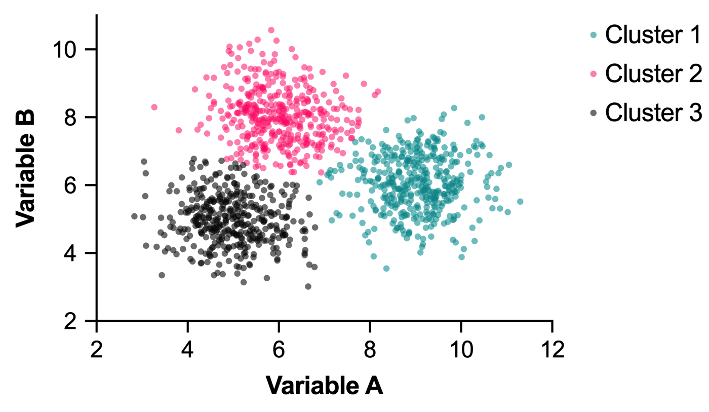
The WCSS calculated for this data grouped into three clusters is reported by Prism as 1468.89. This number will be used a bit later in the calculation of the gap statistic. For now, let’s consider a second data set:

This data is related to the first data set in that they both consist of 1200 points, and they both have the same minimum and maximum values for Variable A and Variable B (in other words, the data represent the same range in the two-dimensional space). The difference with this data is that these data points were simulated to be more or less uniformly distributed throughout this region. The clear grouping of data is no longer visible in this dataset. If we perform K-means clustering on this data using three clusters as we did for the previous data set, we get the following results:

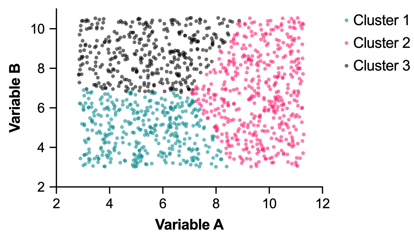
The WCSS calculated for this data grouped into three clusters is 4896.79. If we compare this value to the WCSS calculated for the same number of clusters on the previous data set (1468.89), we see that the WCSS for the previous data set is much smaller than the WCSS calculated for this data set. This suggests that the clusters identified in the first data set are much more compact (smaller dispersion of data within each cluster). Another way to think about this result is to say that the data in the first data set are grouped into clusters better than the corresponding random simulated data on the same variable range.

This is the general intuition behind the gap statistic method: start by comparing how well the input data clusters against randomly simulated data on the same variable range. If a given number of groupings truly exist in the input data, then when those data are grouped into that number of clusters the resulting WCSS (the “WCSS observed”) should be much smaller than the WCSS resulting from clustering of random data from the same variable range into the same number of clusters.

To ensure that this reduction wasn’t a result of random chance, this process can be repeated with numerous additional uniformly distributed datasets, and a WCSS value can be calculated for each of them (the “WCSS expected”). The natural log of these WCSS values is then calculated and the average of these log-transformed values is determined. Then, the difference between log(WCSSexpected) and log(WCSSobserved) for a given number of clusters can be calculated. It’s this difference that is referred to as the “Gap statistic”.

To determine the optimal number of clusters using this gap statistic, the standard deviation of the WCSS values determined for the randomly generated data sets must also be calculated. Then, you compare the gap statistic for “k” clusters with the gap statistic for “k+1” clusters. The optimal number of clusters occurs when the gap statistic for “k” clusters is bigger than the gap statistic for “k+1” clusters minus the standard deviation for “k+1” clusters.

Let’s formalize some of these concepts with math:

where

•k is the number of clusters

•WCSSexpected is the average WCSS across all randomly generated data sets grouped into “k” clusters. Given in Prism as “log(W) expected”

•WCSSobserved is the WCSS of the input data grouped into “k” clusters. Given in Prism as “log(W) observed”

The full calculation of WCSSexpected is given as:

where

•k is the number of clusters

•B is the number of randomly generated data sets

•Wkb* is the WCSS of the “b-th” data set grouped into "k" clusters

Next, the standard deviation that Prism reports and that is used to calculate the optimal number of clusters is actually a scaled standard deviation (to account for simulation error):

where

•k is the number of clusters

•B is the number of randomly generated data sets

•sdk is the standard deviation of the WCSS values across all randomly generated data sets grouped into “k” clusters

Note that Prism uses 100 for the value of B when calculating the gap statistic, and reports the value sk as “SD” in the detailed results for the gap statistic method.

Finally, the optimal number of clusters can be determined as: