Before getting into the details of the values reported by Prism for residuals from Cox proportional hazards, it must be noted that these are NOT residuals in the classic sense. For linear regression (multiple linear regression or simple linear regression) and nonlinear regression, residuals represent the difference between the observed value and the value that is estimated by the model (specifically, the mean value predicted by the model for this observation).
Unfortunately, the concept of residuals in Cox proportional hazards regression does NOT adopt this same definition. Instead, the values presented as residuals in Cox proportional hazards regression are simply metrics that have been proposed and used to answer many of the same questions in Cox regression that classic residuals are used to answer in other types of regression. The sections below provide a brief explanation of each of the residual graphs that Prism offers as part of Cox proportional hazards regression.
Is the proportional hazards assumption valid?
This question is central to the Cox proportional hazards regression analysis (it’s right there in the name!). The general idea is that the occurrence of the event of interest for every individual in the population is governed by a single underlying baseline hazard function, and that the specific hazard rate for each individual at any time point is simply a scaled version of this baseline hazard rate. Another way to think about this assumption is from the point of view of the estimated beta coefficients. For the proportional hazards assumption to be true, these parameter estimates must be constant with respect to time.
To test this assumption, Prism offers two different graphs. The first is a graph of the scaled Schoenfeld residuals vs time/row order. Importantly, there will be one set of scaled schoenfeld residuals for each parameter in the model. This distinguishes Schoenfeld residuals from the other types of residuals that Prism offers for Cox proportional hazards regression (in which there is one residual per observation in the input data). The idea is that, when the scaled Schoenfeld residuals for a given parameter are plotted against time, they should be centered about a horizontal line at zero. If there is a trend in these residuals, it is possible that there is some time-dependence of the parameter estimate with respect to time (thus violating the proportional hazards assumption of the analysis).
The other graph that can be used to examine the proportional hazards assumption is the Log-minus-log plot (plotting Ln(-Ln(S(t))) against time for multiple groups defined in the input data. Using the controls in the parameters dialog, Prism will allow you to specify different groups (defined by predictor variable values) to plot estimated survival curves. When plotting the natural log of the negative natural log of these survival curves (Ln(-Ln(S(t)))) against time, each set of values should be roughly a straight line. Moreover, if the proportional hazards assumption is correct, these lines should be parallel for any given group. Thus, if these lines cross, it’s a strong possibility that the proportional hazards assumption has been violated.
Were there outliers in the observations?
Deviance residuals and Martingale residuals can be plotted against the linear predictor (XB) or the hazard ratio for an observation, while Schoenfeld residuals can be plotted against time or row order to examine the possibility of outliers in the input data.
Deviance and Martingale residuals are both used to identify outliers as individuals who either had an elapsed time to the event of interest much longer than the model predicted, or as individuals who experienced the event of interest much sooner than predicted by the model. For these residuals, large positive values represent individuals that experienced the event of interest sooner than the model predicted, while negative values represent individuals that “survived” longer until the event of interest than the model predicted. The primary difference between these two sets of residuals is their distribution and skew. Martingale residuals have a theoretical maximum value of +1, but can take on negative values of any magnitude, resulting in values that may look like outliers (individuals that survived longer than predicted), but that are not actually outliers. For this reason, it is recommended to use deviance residuals instead. These values are more evenly centered around zero, with a more even spread of values in both the positive and negative directions.
When plotted against time, Schoenfeld residuals can also be used to identify outliers in the data, but these residuals are actually used to discover highly influential observations on the parameters in the model. Like scaled Schoenfeld residuals, there is one set of residual values for each of the parameters in the defined model. Using the Format Graph dialog, the specific residuals to be plotted on the generated graph can be cycled through. For these graphs, residuals with large magnitudes indicate observations that have a large impact on the selected parameter.
Are the predictor variables linear?
Another of the assumptions of the Cox proportional hazards regression model is that there is a linear relationship between the log(hazard rate) and the parameter estimates. Recall that the model for Cox proportional hazards regression is:
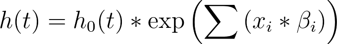
Or alternatively:
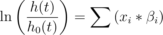
In this arrangement, it can be see that each value of β should have a linear relationship with the log(hazard rate). By plotting either Deviance or Martingale residuals vs the values of the predictor variable values, this linearity assumption can be investigated. For linear predictor variables, these residuals should be roughly centered around zero for any value of the predictor. Trends observed in the residuals over different predictor variable values may suggest departures from linearity. As with using deviance and Martingale residuals to check for outliers in the data, it is again recommended to use deviance residuals when examining the linearity of predictor variables due to their more even distribution around zero.
How good was the fit?
The last type of residual graph that Prism provides for Cox proportional hazards is the Cox-Snell residuals vs. Nelson-Aalen survival estimator of the cumulative hazard rate. Like the Kaplan-Meier estimator of the survival function, the Nelson-Aalen estimator of the cumulative hazard function is a non-parametric estimate of the cumulative hazard rate. The Cox-Snell residuals are defined as follows:
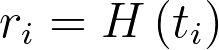
In other words, the Cox-Snell residual for observation i is equal to the estimated cumulative hazard of this observation (this value is reported by Prism on the Individual values tab of the results).
The idea is that if the model fits the data well, plotting the Cox-Snell residuals (values of the cumulative hazard estimated by the model) against the Nelson-Aalen estimator of cumulative hazard (a non-parametric estimate) would result in a straight line. This is actually the case for well-fitted models, and these graphs are often used to demonstrate goodness of fit. But there’s a problem! Many studies have been reported that indicate that it takes a particularly ill-fit model to generate a graph of Cox-Snell residuals vs. the Nelson-Aalen estimator of cumulative hazard that isn’t roughly linear. In other words, just because this graph generates a straight line, this is not confirmation that the model fits the data well.