Parameter estimates
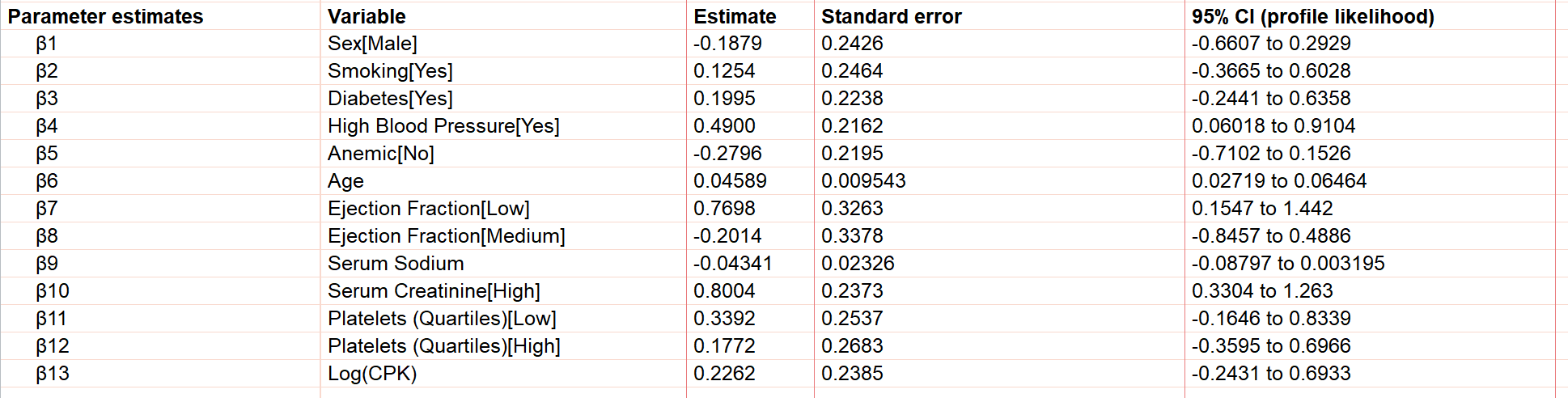
The first section of results that you’ll see are the best-fit values for the regression coefficients (beta coefficients) for the specified model. Note that - unlike some other multiple regression techniques - Cox proportional hazards regression does not include an intercept term (β0). Even if an intercept term were forced into the model, it would simply be “absorbed” by the baseline hazard (h0(t)). Additionally note that when categorical variables are included in the model, these are "dummy coded" automatically, resulting in a separate parameter estimate for every level of the categorical variable other than the reference level. Thus, the results for our model include thirteen separate beta coefficients as shown below:
Interpretation of these parameter estimates is a bit different than in standard multiple linear regression. Consider the Cox proportional hazards model for this analysis:

If we rearrange this equation by dividing the baseline hazard, we get the following:

Finally, if we take the natural logarithm of both sides, we’re left with this form:

Using this form of the equation, it can now be seen that the left-hand side of the equation is the log of the ratio of the hazard rate for a specific individual or group (using the specific predictor variables that correspond to this individual or group), divided by the baseline hazard (which represents the hazard rate when all predictor variables are set to zero or their reference value). This is where the term proportional hazards comes from, since the model in this analysis is actually estimating a ratio of hazards (groups specified with different predictor variables and the baseline group).
Knowing this, we can see that the value of the beta coefficient represents an increase (for positive values) or a decrease (for negative values) in the log-hazard rate. For example, in our results, β1 (Sex[Male]) equals -0.1879. This means that when compared to women, the log-hazard rate for men is decreased by 0.1879 at all time points. The value of β6 (Age) is 0.04589. This means that for every year increase in age of an individual, the log-hazard rate increases by 0.04589.
Hazard ratios
Direct interpretation of beta coefficients is complicated since these correspond to changes in the log-hazard rate, while it’s generally easier to understand changes on a linear scale as opposed to a logarithmic scale. As such, the next section of the results is the Hazard ratios.
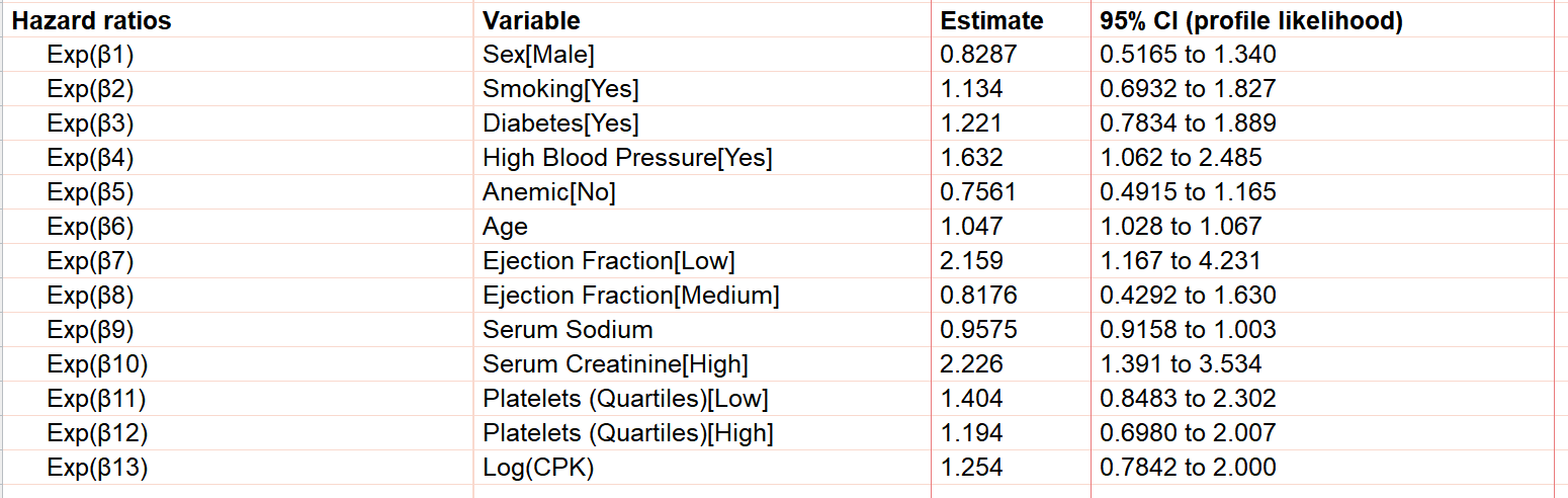
A more detailed discussion of the relationship between parameter estimates and hazard ratios can be found here, but essentially a hazard ratio represents how many times greater (or smaller) the hazard rate is when the predictor variable associated with the hazard ratio is increased by one. Again, using Age in the example above, we see that the hazard ratio is equal to 1.047. This means that for every year increase in age of a participant, their hazard ratio would increase by a multiple of 1.047. Mathematically speaking, hazard ratios are simply the exponentiated beta coefficient (e.g. the hazard ratio of 1.047 for Age is equivalent to exp(0.04589), where 0.04589 is the beta coefficient for Age in this model).
Taking all of this into account, we can see that the general conclusion of this model so far is that we would expect that older individuals with poor heart function (low ejection fraction), high blood pressure, and poor kidney function (high serum creatinine) are predicted to have an increased hazard rate (and thus a decreased survival time). Note also that although the hazard ratio for Age seems relatively small (1.047 for Age compared to 2.226 for high Serum Creatinine, for example), this is the effect of age per year. This means that the hazard rate would only increase by a factor of 1.0471 = 1.047 for a one year increase in age, but would increase by a factor of 1.04710 = 1.58 for a ten year increase in age!
P values
By default, P values for parameter estimates aren’t given in the results, and thus will not be discussed in detail here. However, if you’d like to include P values in the tabular results of the analysis, you may do so by enabling this option on the Options tab of the analysis dialog. More information on how to interpret these P values can be found here.
Model diagnostics
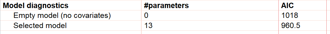
The next section of the tabular results for Cox proportional hazards regression provides information that compares the specified model with a model containing no predictor variables (covariates). By default, the values displayed here include the number of parameters for each of the models, and the Akaike’s Information criterion (AIC) value. Other diagnostic values can be added on the Options tab of the analysis dialog.
The AIC values listed in this section allow you to quickly assess if the model specified in the analysis does a better job at fitting the data than the empty (null) model. The way that the AIC values are calculated is a little complex, but using these values to compare two models is actually straightforward: a smaller AIC indicates a better model fit. With values of 1018 for the model with no covariates and 960.5 for the model specified in the analysis, we can determine that the specified model does a better job of describing the observed data.
Data summary
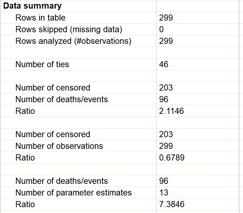
The last section on the tabular results page for Cox proportional hazards regression simply provides a detailed summary of the input data, including the number of rows of data in the input data table, the number of rows that were skipped, and the difference between these two values resulting in the number of observations included in the analysis. Next, this section reports the number of ties (observations with events that possess the same elapsed time). After this, the number of censored observations and the number of observations with a recorded death/event of interest are provided. From these two values, the ratio of censored observations to events is reported. Depending on the event being studied, this ratio may vary considerably (when the event is relatively uncommon, the ratio of censored observations to events may be large such as in this example; when the event is common, the ratio may be very small since most observations will result in the event occurring).
Additionally in this section, the number of censored observations and the total number of observations are repeated along with the ratio of these two values (providing the fraction of observations used in the analysis that were censored). Finally, the number of observations with a recorded death/event of interest is repeated along with the total number of parameter estimates and the ratio of these two values. Generally, this ratio of the number of events per parameter should be around ten.
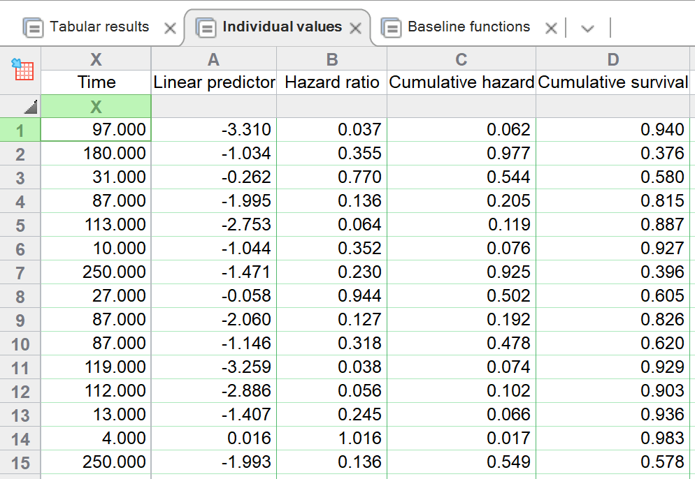
Individual values
There are two other tabs of results that are generated by default for Cox proportional hazards regression. The first of these is the Individual values tab. As the name implies, this table of results provides calculated values for each individual (row) in the input data table. The elapsed time for each individual is included in this table, along with the linear predictor, hazard ratio (exp[linear predictor]), and the cumulative hazard and cumulative survival calculated from the generated model for each individual at the reported elapsed time. Specific details on how these values are calculated can be found on this page in the guide.
Baseline values
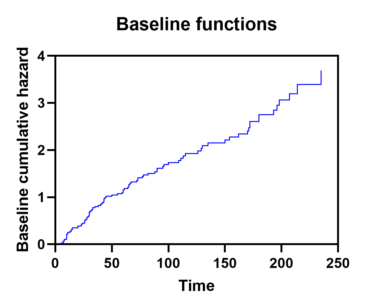
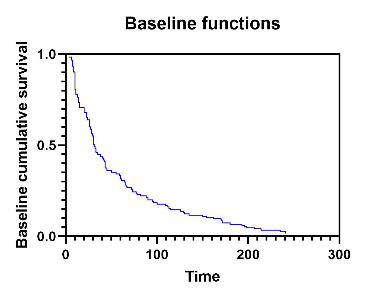
In addition to providing estimated values for each of the specific observations (rows) in the input data table, Prism also generates a table of baseline values for both the baseline cumulative hazard (H0(t)) and the baseline cumulative survival (S0(t)). Unlike the Individual values table, this table includes one row for each unique time in the input data, and is sorted by these time values in ascending order.
The calculation of baseline cumulative hazard and baseline cumulative survival is covered on a separate page, but it should be noted that this table is used to generate the graph of baseline values that can be set to display either the baseline cumulative hazard or the baseline cumulative survival (both examples for this analysis shown below).
Importantly, these baseline graphs can then be used to build estimated survival/hazard curves for specified populations using the parameter estimates (or hazard ratios) for each predictor variable.
Residual graphs
By default, Prism will generate three different residual graphs:
•Scaled Schoenfeld residuals vs time/row order
•Deviance residuals vs linear predictor/HR
•Deviance residuals vs covariate
Each of these can be used to examine a different aspect of the model fit.
Scaled Schoenfeld residuals vs time/row order
The main use of this graph is to test the proportional hazards assumption of the specified model. A set of scaled Schoenfeld residuals is generated for each parameter included in the model (in our case, β1 through β13). By plotting these residuals on the Y axis against time on the X axis, we expect there to be no significant trend in the plotted data. Each of the different sets of residuals can be examined on the same graph (changing the variable plotted on the Y axis using the Format Graph dialog), and any strong trends in these residuals suggests that the proportional hazards assumption may have been violated. In our case, it appears as though this assumption is valid (examples below given for β1:Sex[Male] and β6:Age).


Deviance residuals vs linear predictor/HR
This graph of residuals can be used to examine the data for any potential outliers. These residuals will be centered around zero. Extremely large or extremely small values represent potential outliers in the data. These points indicate subjects that experienced the event of interest much sooner than the model predicted (extremely large positive residuals) or much later than the model predicted (extremely large negative residuals). Using the Format Graph dialog (double click in the graphing area to open), the linear predictor or Hazard ratio for each observation (values provided on the Individual values tab of results) can be plotted on the X axis. The only difference between these two is scaling (since the hazard ratio is the exponentiated linear predictor). Note that the large dense cluster of points in the lower left region of the graph below is due to a high proportion of censored observations in the data set. By definition, censored observations must have negative deviance residuals (based on the mathematical equations used to calculate the residuals, not shown here). Intuitively, this makes sense though. An observation that is censored has no observed event time. Thus, these observed event times cannot be earlier than the model predicts (the requirement for a deviance residual to be positive). Thus, all censored observations must have negative deviance residuals.

Deviance residuals vs covariate
These residual plots are used to test the linearity assumption of each of the covariates. When plotting the deviance residuals against each of the covariates in the model, it is expected that these residuals would be roughly centered about zero. Trends in these graphs may suggest that the linearity assumption of the selected covariate has been violated. Note that currently, Prism is only able to display continuous predictor variables (covariates) on the X axis for these graphs. The graph for deviance residuals vs Age for our model is shown below, and displays no obvious trend, suggesting that the assumption of linearity in this predictor variable is not violated.

Estimated survival graphs
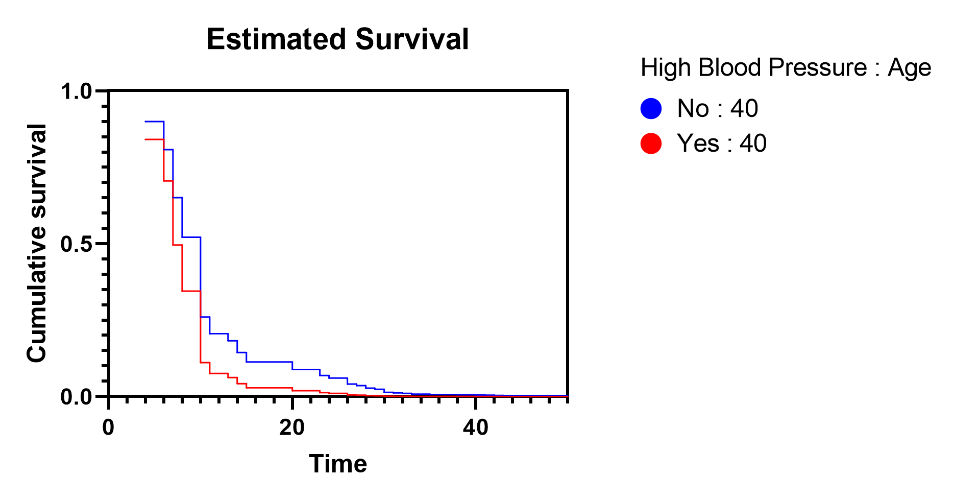
The last graph generated by the analysis that we’ll look at contains the estimated survival curves for the groups that we specified on the Graphs tab of the analysis parameters dialog. Using the options on this tab, we had selected the variables of High blood pressure (with both “Yes” and “No” values selected) and Age (with a value of 40). Prism used this information along with the baseline survival curve (discussed on this page) to generate estimated survival curves for two populations:
•A population with high blood pressure and age 40
•A population with low blood pressure and age 40
The graph that Prism generates shows us a number of important concepts. First, we see that those with high blood pressure are estimated to have a lower survival probability than those without high blood pressure. This matches with the value of the parameter estimate (and hazard ratio) that we saw earlier for this same predictor variable. A positive parameter estimate (β4 = 0.490) resulting in a hazard ratio greater than one (HR=1.632) indicates a higher hazard (and lower survival probability) for individuals with high blood pressure compared to those without high blood pressure.
The other very important concept that these estimated survival curves demonstrate is the assumption of proportional hazards. This assumption states that the hazard of every individual is proportional to some baseline hazard. This assumption can be shown visually using the estimated survival curves for a range of different age values. The following graph includes the baseline survival curve along with five different curves representing different values of age.
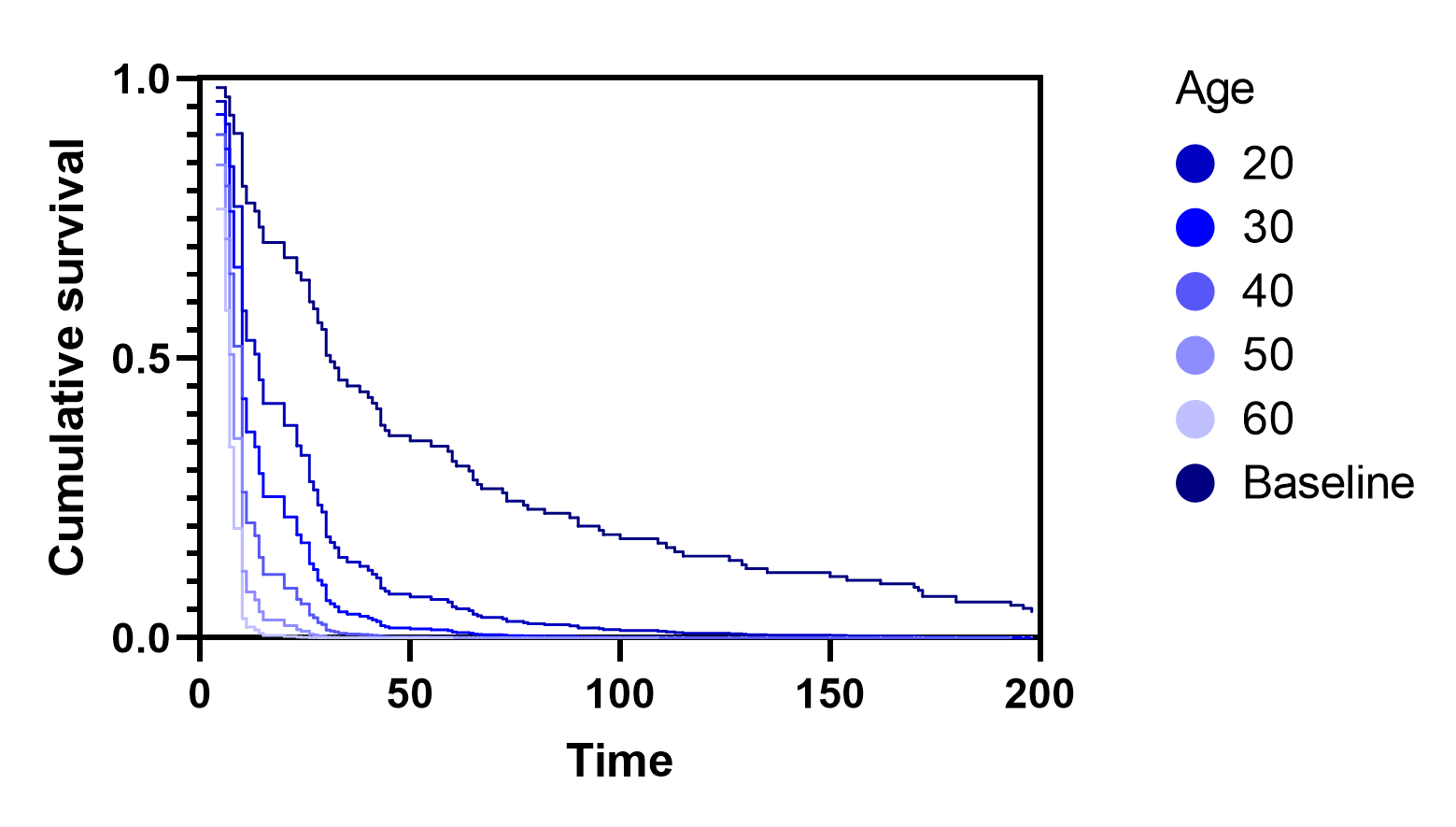
As can be seen, each of these survival curves adopts the same general shape, with the specific values of survival probability at any given time being proportional to the baseline survival probability at that time point.