The final tab shown by default by PCA with Prism is the PC Scores tab. The concept of “scores” for each principal component was already briefly discussed when looking at eigenvalues and eigenvectors. As mentioned before, PCs are simply linear combinations of the variables in the dataset, with the coefficients of these linear combinations being given by the eigenvector for the PC. In our example, consider PC1. The linear combination of variables for this component (using the values of the eigenvector for PC1) is:

PC1=0.552*(Variable A)+0.553*(Variable B)-0.227*(Variable C)+0.181*(Variable D)-0.530*(Variable E)

To calculate the “Scores” for PC1, we simply plug in the values from the standardized (or centered) data into this equation. Each row of data corresponds to a single “score” for each PC. For example, the first row of standardized data in this analysis is:

 

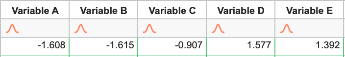
Thus, to calculate the first score for PC1:

PC1 = 0.552*(-1.608) + 0.553*(-1.615) - 0.227*(-0.907) + 0.181*(1.577) - 0.530*(1.392) = -1.981

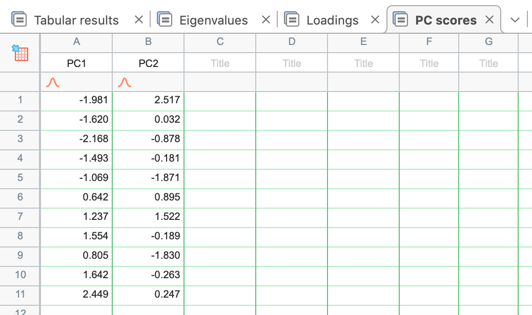
The remaining scores for PC1 and the scores for all other selected components can be calculated in the same way, resulting in the PC scores table presented by Prism:

PC Scores results table

 

Subsequently, these scores can be used to create “Score plots” for the analysis. These graphs will be described in more detail in a different section, but the general idea is that these score plots allow for the projection of the original data into the two-dimensional space defined by two of the selected principal components. This is a very visual representation of the dimensionality reduction goal of PCA.

PC Scores plot (PC1 vs PC2)