How Do I Perform a Dose-Response Experiment?

Non-linear regression analysis is used to evaluate the results of a dose-response experiment. In these experiments, an organism (cell line or animal model) is exposed to a stimulus/stressor (drug) and the response (outcome) is measured. The analysis consists of plotting the drug dose or concentration vs. response and applying a non-linear regression model. The result is a sigmoidal curve.

Here, we discuss the response and dose values, how to apply a non-linear regression model and evaluate your results.

Learn more about dose-response curves with Prism curve-fitting guides. 

 

What do the X and Y values represent?

In pharmacology, a dose-response experiment determines the effects of a drug on cells grown in vitro. For example, a dose-response experiment studies how well a drug decreases the growth of tumors grown in cell culture.

This analysis consists of plotting X values that represent the drug concentrations or function of concentrations (log concentration) vs. Y values representing the response. The outcome is a sigmoidal curve (dose-response curve) with bottom and top plateaus (see below). It must be noted that these measured responses are end-point measurements. In other words, the response is measured after treating the biological system with different concentrations of the drug. The response is not measured at different times after treating the biological system with a single drug concentration.  

 

X values

X values are concentrations (doses) of a drug used in the experiment. In pharmacology, four different classes of drugs used in dose-response experiments include:

 

1. Agonist – Causes a stimulatory (response increases as drug concentration increases) or inhibitory (response decreases as drug concentration increases) response. A Full agonist causes the maximum response.

2. Partial agonist – Elicits a response but cannot elicit the maximum response.

3. Inverse Agonist – Produces the opposite response than that of the agonist. Reduces the preexisting basal response (response seen in the absence of any drug).

4. Antagonist – Inhibits the action of the agonist.

Read more about agonist and antagonist equations.

Y values

Y values are the response measured in intervals. The response can decrease as drug increases (downward sigmoidal curve) or the response can increase as drug increases (upward sigmoidal curve), see below.

 

• In dose-response analysis, the Y values are assumed to follow Gaussian or “normal” distribution at any given concentration (X value). If you were to graph the probability distribution of variable points (Y) at any X value, the curve would resemble a bell-shaped curve. The peak of the bell would be the most probable event. This is a statistical concept and not to be confused with the sigmoidal curve resulting from the analysis.  

• Y values can be transformed into different units by multiplying or dividing by a constant. For example, in an assay you may measure the fluorescence but would like to plot concentration units. Knowing before-hand the relationship between the amount of fluorescence generated and the concentration of target in a sample allows you to convert measured fluorescence response values to corresponding concentration values simply by dividing by a constant.

• The response can also be transformed through normalization. For example, the response may be changed to percentage-with the maximum signal converted to a response of "100" and the minimum signal converted to a response of "0"-allowing comparison of different experiments. We discuss transformation and normalization later.

Number, range and spacing of concentrations

Considering the number, range and spacing of the concentrations leads to better interpretation of the drug effect.

• Number of X values - Usually, it is recommended that you plot 5-10 concentrations distributed well through a broad range allowing for measurements to generate the bottom plateau, the top plateau and the central part of the curve (2). The more values, the higher analysis quality.

• Range - Applying the logarithmic function to concentrations prior to analysis is advantageous when the concentrations increase exponentially, such as 1, 10, 100, 1000. It allows better visualization of the shape of the curve by reducing the dispersion of the data.

• Taking the logarithm facilitates analysis by spreading data points equally.

 

Non-linear regression analysis

The complexity of biological systems results in a non-linear dose-response relationship requiring consideration of multiple parameters during analysis. Dose-response analysis is a type of curve-fitting analysis that uses non-linear regression—an iterative mathematical model that fits your data and considers these parameters—to accurately characterize the dose-response relationship.

Nonlinear regression can determine a drug’s potency (EC50 or IC50), find best-fit values, compare results from different experiments and interpolate unknowns from a standard curve. For example, you can study the effect of treating cells with an agonist in the presence and absence of an antagonist (an inhibitor) as seen below.

 

However, this analysis has multiple assumptions and limitations.

Assumptions of non-linear regression

• The exact value of X is known. Y values are the only values that have errors (scatter).

• Variability of Y values at X follows Gaussian bell-shaped distribution.

• Uniform variance: The amount of scatter (standard deviation) is the same along the curve. Try weighting tools in Prism to resolve non-uniform variance. 

• All observations (Y values) are independent (3).

Limitations

• Biological systems are very complex and non-linear regression analysis may not fully characterize the dose-response relationship. For example, EC50 may be determined by both the affinity and the efficacy of the drug. Prism offers various tools to determine affinity and efficacy.

o   The affinity is how well the drug binds to the receptor.

o   The efficacy is the ability of the drug to evoke a response once bound. Efficacy can vary widely.

• The results may vary depending on the concentration range and cell/tissue type being used.

• The initial values of the parameters used also affects the analysis and may need constraining to increase analysis quality.

 

Using the four parameter logistic (4PL) regression model

The Hill Equation or 4 parameter logistic (4PL) model is a standard model often used in dose-response curve analysis.

What is the Four Parameter Logistic (4PL) Regression Model?

This non-linear regression model estimates 4 different parameters: Bottom (minimum response), Top (maximum response), Hill Slope and EC50. The parameters may be constrained (discussed later).

Equation and parameters of the 4PL regression model

 

X = log of dose or concentration

Y= response

1. Minimum response (Bottom). The Y value at the minimal curve asymptote (Bottom plateau).

2. Maximum response (Top). The Y value at the maximum curve asymptote (Top Plateau)

3. Slope factor (also called Hill Slope). Defines the steepness of the dose-response curve. If the Hill slope <1, the sigmoidal curve is shallower. If Hill slope > 1 then the sigmoidal curve is steeper (see below). Constraining the slope value to 1.0 (standard Hill slope) or using a variable slope depends on the system and number of observations. If the number of observations is low, set the slope to 1.0. A variable slope is recommended for receptor-ligand binding assay analysis.

4. EC50 and IC50 values

EC50 (effective concentration) is the concentration of drug that elicits a response halfway between the baseline and maximum response (dose-response curves going upward) as seen below. IC50 (inhibitory concentration) is the concentration of a drug that elicits a response halfway between the maximum response and the minimum response, in downward-sloping dose-response curves. EC50 is influenced by a drug’s affinity and efficacy (3). 

Illustration of EC50 value.

 

Relative and absolute IC50/EC50

In ideal cases, the dose-response curve extends between the control values, and the IC50 does not change whether you fit all the data without the control values, set the Top and Bottom equal to the mean of the blanks or use control values.

However, the dose-response curve may not extend between the controls (the NS controls are considerably lower than the Bottom plateau) as seen below. So, how do we calculate the IC50?

The relative IC50 is estimated by considering the Bottom and Top plateaus obtained by implementing the 4PL model and ignoring NS control values (1).  Whereas, absolute IC50 are obtained considering the control values and determining the point at the curve where 50% inhibition is observed (see below).

This figure shows the relative and absolute IC50 values when NS controls fall below the bottom plateau.

 In general, dose-response analysis uses the relative IC50 or EC50.  

 

Is your data ready for curve-fit analysis?

Preparing your data for analysis may include manipulation through transformation, normalization, data smoothing or deleting outliers. Once your data is ready to be analyzed, you can follow these steps to fit your data to a model.

Transformation

Transformation is the application of a mathematical function to X or Y values. X is often transformed by taking the log of concentrations prior to curve-fitting analysis. This transformation of X does not affect the standard errors or confidence intervals and is advantageous as noted earlier. 

However, graphing the logarithm of X is not the same as graphing the logarithmic axis. Specifically, using a logarithmic axis only changes the appearance of the graph. The data itself does not change. Thus, when performing analyses, you will be performing the analysis on the original data, not transformed data.

Y can be also be transformed by dividing/multiplying by or subtracting a constant without affecting parameters or confidence intervals. Changing the Y units through transformation may facilitate curve-fit analysis.

Normalization

Transformation by normalization (usually diving by a constant and subtraction of baseline from all response values) changes the range of responses so that they fit between 0. and 1.0 or 0% and 100% (3). Then, you can fit all the data. This transformation does not change the Hill Slope or the EC50/IC50 (Top and Bottom plateaus will change) and enables a comparison of results (EC50) from multiple experiments. 

Learn about the advantages and disadvantages of normalizing data with Prism.

Smoothing

Smoothing data generates a rolling average and creates the impression of a trend. It is not advisable to smooth your dose-response data (3). See the GraphPad Curve Fitting Guide for additional information.

Outliers

Outliers are Y values that may be perceived as being too far from other response values. Do not exclude outliers from the analysis without investigating the cause. Learn how to exclude outliers with Prism.

 

Evaluating and troubleshooting dose-response curve analysis

Analysis is followed by evaluation of the dose-response curve and parameters whether it is a new or established assay. The goal is to find the best model.  

Is the curve sigmoidal?

• Is the dose-response complete? Incomplete dose-response curves do occur but an IC50 value can still be obtained using different approaches (see figure below).

The dose-response curve on the left is incomplete. On the right, control values (green dots) are used to obtain an IC50 value.

• Does the generated curve align (comes near) with the data points? If the curve appears to be biphasic or non-sigmoid, then your dose-response experiment may require other non-linear regression models (3).

 

Does the EC50 or IC50 value make sense?

EC50 (or IC50) should be within range of your data, near the middle of the curve. If these values are not appropriate, it might be useful to constrain some of the parameters.

Top and bottom plateaus

Check that plateaus are reasonable. The maximum plateau should not be considerably higher than your highest data point. However, some stimulation 4PL models do result in the maximum plateau being considerably higher than the highest data point because data was not collected at the highest doses. In this case, the full sigmoidal curve will not be visualized. This is common and may be resolved by collecting more data points. 

Standard error of parameters

Non-linear regression calculates standard error of different parameters. Standard error is particularly important in the calculation of 95% confidence intervals.

Inspect the 95% confidence interval and 95% prediction band

The 95% confidence interval means you can be 95% confident that the true curve falls inside that range (see below). The narrower the confidence band, the better. The 95% prediction band represents the idea that 95% of future results (if you were to perform the same experiment again) would fall within that interval (see below) (3).

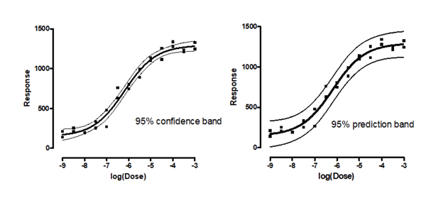
The 95% confidence band (left) is usually narrower than the 95% prediction band (right).

 

When do I constrain parameters?

Depending on the biological system and the experiment, defining the dose-response relationship and obtaining an accurate EC50 may require constraining parameters (fixing to a constant value).  

•  In the case of the Hill Slope, your dose-response analysis may yield accurate results by constraining the slope to 1.0. This is applicable especially when you have many data points.

• Constrain the Bottom plateau to 0 when the response is bounded below by 0. The dose-response curve can bottom out at some non-zero value when low drug concentrations don't change the response. It is not necessary to use the curve-fit analysis to find a best-fit value for the Bottom plateau. May also constrain to a Control value. 

• The Top plateau may be constrained to a Control value. However, if no control exists and you have many data points to possibly define the plateau, then the Top plateau may be obtained through best-curve fit analysis.

 Explore the Constrain tab in Prism. 

The ambiguous case

You have analyzed the data, but the model can’t estimate all the parameters. Perhaps you did not collect enough points and the sigmoidal curve looks incomplete (as seen in Evaluating and Troubleshooting your dose-response analysis section).

In this case, you can constrain one or more parameters (to control values, for example), collect more data points or share the same parameters across different datasets. 

Prism helps you identify ambiguous fits.

 

Can I compare different models?

The Compare tab in Prism may be useful when trying to do the following:

•  Find what model fits a data set best by comparing two models. For example, compare the 5PL model to a 4PL model or 3PL model. 

•  To determine if best-fit values of specific parameters differ between data sets. For example, compare EC50 values for different agonists. 

•  Compare the fit of a best-fit value of a parameter vs. a theoretical value. For example, using a variable slope vs. a standard slope.

Learn more about how to analyze dose-response on Prism Academy.

 

References 

1. Sebaugh, J. L. (2011). Guidelines for accurate EC50/IC50 estimation. Pharmaceutical Statistics, 10(2), 128-134. doi:10.1002/pst.426.

2. Coussens, N. P., Sittampalam, G. S., Guha, R., Brimacombe, K., Grossman, A., Chung, T. D., . . . Austin, C. P. (2018). Assay Guidance Manual: Quantitative Biology and Pharmacology in Preclinical Drug Discovery. Clinical and Translational Science, 11(5), 461-470. doi:10.1111/cts.12570. 

3. Motulsky, H., & Christopoulos, A. (2010). Fitting models to biological data using linear and nonlinear regression: A practical guide to curve fitting. Oxford: Oxford Univ. Press.

   1. The 95% confidence interval is a range of values constructed such that - were you to repeat the exact same experiment many times - 95% of these ranges would include the true curve (though this true curve would still be unknown).