The field of statistics attempts to “quantify uncertainty” found in data. Confidence intervals, prediction intervals, and tolerance intervals are all ways of accomplishing this. It is important to understand the differences between these intervals and when it’s appropriate to use each one. After describing each type of interval, an example is given where all three are used.

Confidence intervals, prediction intervals, and tolerance intervals are three distinct approaches to quantifying uncertainty in a statistical analysis. The discussion below explains these three types of intervals for the simple case of sampling from a Gaussian distribution. 

Improve the performance of your analysis with Prism. Try Prism for free.

 

Confidence Intervals

Confidence intervals tell you how well you have determined a parameter of interest, such as a mean or regression coefficient. 

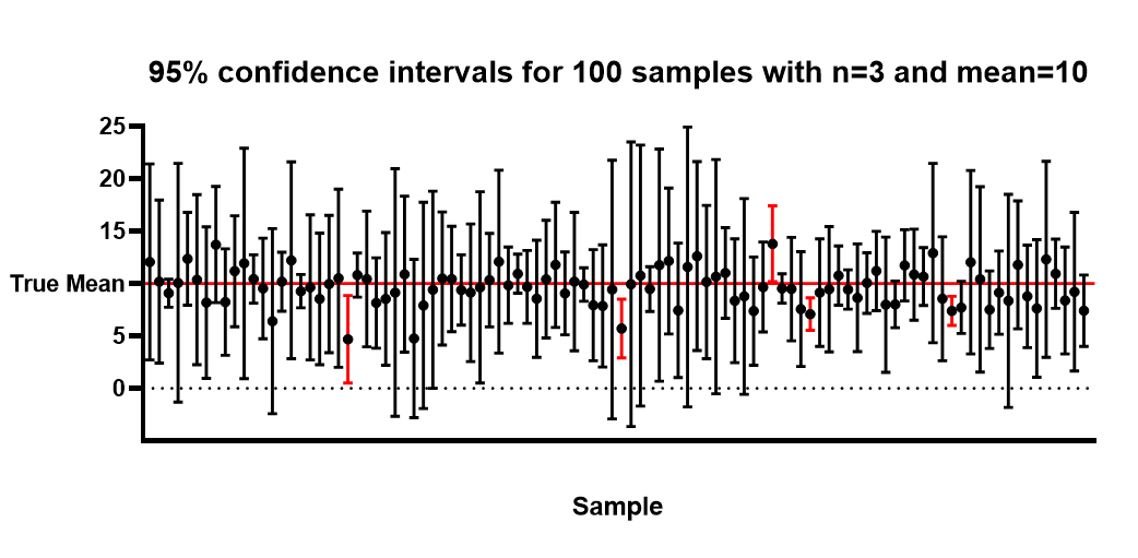
Assume that the data are randomly sampled from a Gaussian distribution and you are interested in determining the mean. If you sample many times, and calculate a confidence interval of the mean from each sample, you'd expect 95% of those intervals to include the true value of the population mean. The diagram below shows 95% confidence intervals for 100 samples of size 3 from a Gaussian distribution with true mean of 10. Note that 95 out of 100 intervals include the value 10. This is what we would expect to see. You won’t know if the particular interval of interest to you captures the true mean, but you can expect 95% of the intervals you calculate to capture the true population parameter.

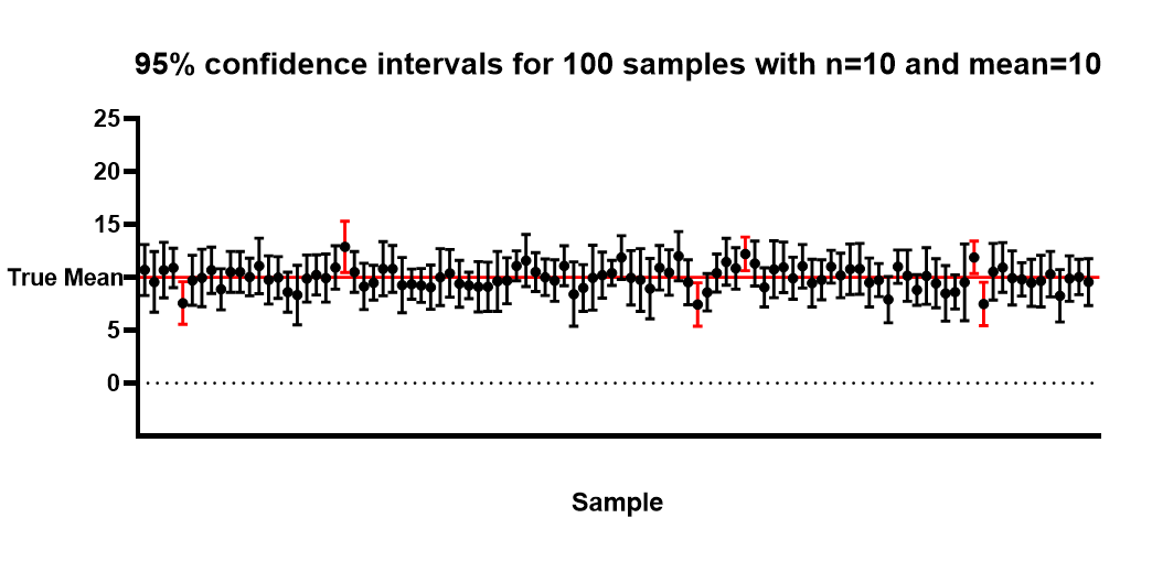
If you increase the sample size, you will see a noticeable decrease in the width of the confidence interval. The diagram below shows 95% confidence intervals for 100 samples of size 10 from a Guassian distribution with true mean of 10. Note that 94 out of 100 intervals capture 10. Due to sampling variation, in a random set of 100 confidence intervals, you won’t always have exactly 95 out of 100 intervals capture the true population parameter.

Asymptotically (as the sample size approaches infinity), the width of the interval will collapse to a single value which is the true population mean. You can see this in the formula for the confidence interval: Average t*Stdev*(1/sqrt(n)), where t is a tabled value from the t distribution which depends on the confidence level and sample size. As the sample size (n) approaches infinity, the right side of the equation goes to 0 and the average will converge to the true population mean. The is not the case for Prediction and Tolerance intervals. The key point is that the confidence interval tells you about the likely location of the true population parameter and, as the sample size increases, the interval eventually converges to a single value, the true population parameter.

Compute confidence intervals with Prism. Start your free trial today.

 

For more information on confidence intervals, watch this video by CrashCourse

 

Prediction Intervals

Prediction intervals tell you where you can expect to see the next data point sampled. Assume that the data are randomly sampled from a Gaussian distribution. Collect a sample of data and calculate a prediction interval. Then sample one more value from the population. If you repeat this process many times, you'd expect the prediction interval to capture the individual value 95% of the time. 

Prediction intervals must account for both the uncertainty in estimating the population mean, plus the random variation of the individual values. So a prediction interval is always wider than a confidence interval. Also, the prediction interval will not converge to a single value as the sample size increases. You can see this in the formula for the prediction interval: Average t*StDev*(sqrt(1+(1/n))), where t is a tabled value from the t distribution which depends on the confidence level and sample size. As the sample size (n) approaches infinity, the right side does not converge to zero, which is one way to distinguish it from a confidence interval. The key point is that the prediction interval tells you about the distribution of individual values, as opposed to the uncertainty in estimating the population mean and will not converge to a single value as the sample size increases.

 

Tolerance Intervals

Before moving on to tolerance intervals, let's define that word 'expect' used in defining a 95% prediction interval. If you were to simulate many prediction intervals, some would capture more than 95% of the individual values and some would capture less, but on average, they would capture 95% of the individual values. 

What if you want to be 95% sure that the interval captures at least 95% of the population? Or 90% sure that the interval captures at least 99% of the population? These questions are answered by a tolerance interval. To compute, or understand, a tolerance interval you have to specify two different percentages. One expresses how sure you want to be (confidence level), and the other expresses what fraction of the population the interval will contain (population coverage). 

If you set the first value (confidence level) to 50%, then a tolerance interval is essentially the same as a prediction interval. If you set the confidence level to a higher value (say 90% or 99%) then the tolerance interval is wider than a prediction interval. As with prediction intervals, tolerance intervals will not converge to a single value as the sample size increases. The formula for a tolerance interval is Average k*StDev, where k is a tabled value based on the sample size and confidence level.

 

Distribution Assumption

Prediction and tolerance intervals are more affected by departures from the Gaussian distribution than confidence intervals. This is because prediction and tolerance intervals predict where individual values will fall. Confidence intervals are based on the distribution of statistics, such as average or standard deviation, which are typically well approximated by a Gaussian distribution (the approximation gets better as the sample size increases).

 

Example

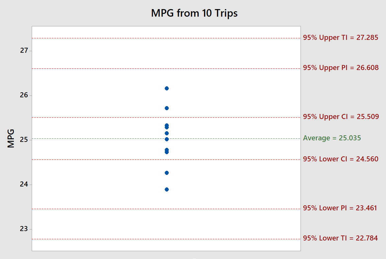
The 2016 Toyota Camry has an advertised city MPG of 25. This car model was driven to and from work 10 times over a two week period. The MPG was recorded after each round trip. The graph below shows the distribution of values from these 10 trips.

The 95% confidence interval for the mean mpg is 25.035 0.475 or (24.560 , 25.509). The 0.475 value is referred to as the margin of error. This confidence interval can be compared to the advertised MPG of 25 to see if this particular Toyota Camry is performing as expected. Since 25 mpg is captured by the interval, the difference between the average of these 10 trips and the advertised MPG is within the margin of error.

 

 

 

You can create this confidence interval yourself by downloading Prism (or opening it if you already have a copy) and completing these steps:

1. Choose Column data table from the left side panel.
2. Choose Enter or import data into a new table and select Enter replicate values, stacked into columns.
3. Click Create. 
4. In the first column enter 25.72, 25.29, 25.15, 25.02, 25.33, 24.73, 26.16, 24.27, 24.78, 23.89.
5. Click Analyze.
6. Select Column analyses > Descriptive statistics.
7. Click OK and select CI of the Mean.
8. Click OK.

In the results table, the 95% confidence interval for the mean is reported as (24.56 , 25.51).

The 95% prediction interval lets you know if you have enough gas for the next trip to work. You can be 95% confident the MPG on the next trip will fall between 23.461 and 26.608. So if you have 1 gallon left in your tank and your work is 23 miles round trip, you can be highly confident you won’t run out of gas on your next trip (although you’d better fill-up on your way home for the next day). 

Finally, the 95%/95% tolerance interval lets you know, at the 95% confidence level, at least 95% of the future trips will have an MPG between 22.784 and 27.285. So if you always start the day with 1 gallon of gas in your tank and your work is 22 miles round trip, you can be highly confident that you will have enough gas for at least 95% of the future round trips.

Since running out of gas can be a costly and time consuming mistake, you probably want to increase the prediction interval and tolerance interval coverage to something more like 99.9%. 

 

Test your understanding of Statistical Intervals

Which type of interval 

• converges to a single value as the sample size increases?
• is the widest of the three types of intervals?
• Is least affected by departures from a Gaussian distribution?

Answers: CI,TI,CI

Start your free trial of Prism today.