The Ultimate Guide to T Tests

The ultimate guide to t tests

The t test is one of the simplest statistical techniques that is used to evaluate whether there is a statistical difference between the means from up to two different samples. The t test is especially useful when you have a small number of sample observations (under 30 or so), and you want to make conclusions about the larger population.

The characteristics of the data dictate the appropriate type of t test to run. All t tests are used as standalone analyses for very simple experiments and research questions as well as to perform individual tests within more complicated statistical models such as linear regression. In this guide, we’ll lay out everything you need to know about t tests, including providing a simple workflow to determine what t test is appropriate for your particular data or if you’d be better suited using a different model.

What is a t test?

A t test is a statistical technique used to quantify the difference between the mean (average value) of a variable from up to two samples (datasets). The variable must be numeric. Some examples are height, gross income, and amount of weight lost on a particular diet.

A t test tells you if the difference you observe is “surprising” based on the expected difference. They use t-distributions to evaluate the expected variability. When you have a reasonable-sized sample (over 30 or so observations), the t test can still be used, but other tests that use the normal distribution (the z test) can be used in its place.

Sometimes t tests are called “Student’s” t tests, which is simply a reference to their unusual history.

It got its name because a brewer from the Guinness Brewery, William Gosset, published about the method under the pseudonym "Student". He wanted to get information out of very small sample sizes (often 3-5) because it took so much effort to brew each keg for his samples.

When should I use a t test?

A t test is appropriate to use when you’ve collected a small, random sample from some statistical “population” and want to compare the mean from your sample to another value. The value for comparison could be a fixed value (e.g., 10) or the mean of a second sample.

For example, if your variable of interest is the average height of sixth graders in your region, then you might measure the height of 25 or 30 randomly-selected sixth graders. A t test could be used to answer questions such as, “Is the average height greater than four feet?”

How does a t test work?

Based on your experiment, t tests make enough assumptions about your experiment to calculate an expected variability, and then they use that to determine if the observed data is statistically significant. To do this, t tests rely on an assumed “null hypothesis.” With the above example, the null hypothesis is that the average height is less than or equal to four feet.

Say that we measure the height of 5 randomly selected sixth graders and the average height is five feet. Does that mean that the “true” average height of all sixth graders is greater than four feet or did we randomly happen to measure taller than average students?

To evaluate this, we need a distribution that shows every possible average value resulting from a sample of five individuals in a population where the true mean is four. That may seem impossible to do, which is why there are particular assumptions that need to be made to perform a t test.

With those assumptions, then all that’s needed to determine the “sampling distribution of the mean” is the sample size (5 students in this case) and standard deviation of the data (let’s say it’s 1 foot).

That’s enough to create a graphic of the distribution of the mean, which is:

Notice the vertical line at x = 5, which was our sample mean. We (use software to) calculate the area to the right of the vertical line, which gives us the P value (0.09 in this case). Note that because our research question was asking if the average student is greater than four feet, the distribution is centered at four. Since we’re only interested in knowing if the average is greater than four feet, we use a one-tailed test in this case.

Using the standard confidence level of 0.05 with this example, we don’t have evidence that the true average height of sixth graders is taller than 4 feet.

What are the assumptions for t tests?

1. One variable of interest: This is not correlation or regression, where you are interested in the relationship between multiple variables. With a t test, you can have different samples, but they are all measuring the same variable (e.g., height).
   
2. Numeric data: You are dealing with a list of measurements that can be averaged. This means you aren’t just counting occurrences in various categories (e.g., eye color or political affiliation).
   
3. Two groups or less: If you have more than two samples of data, a t test is the wrong technique. You most likely need to try ANOVA.
   
4. Random sample: You need a random sample from your statistical “population of interest” in order to draw valid conclusions about the larger population. If your population is so small that you can measure everything, then you have a “census” and don’t need statistics. This is because you don’t need to estimate the truth, since you have measured the truth without variability.
   
5. Normally Distributed: The smaller your sample size, the more important it is that your data come from a normal, Gaussian distribution bell curve. If you have reason to believe that your data are not normally distributed, consider nonparametric t test alternatives. This isn’t necessary for larger samples (usually 25 or 30 unless the data is heavily skewed). The reason is that the Central Limit Theorem applies in this case, which says that even if the distribution of your data is not normal, the distribution of the mean of your data is, so you can use a z-test rather than a t test.

How do I know which t test to use?

There are many types of t tests to choose from, but you don’t necessarily have to understand every detail behind each option.

You just need to be able to answer a few questions, which will lead you to pick the right t test. To that end, we put together this workflow for you to figure out which test is appropriate for your data.

Do you have one or two samples?

Are you comparing the means of two different samples, or comparing the mean from one sample to a fixed value? An example research question is, “Is the average height of my sample of sixth grade students greater than four feet?”

If you only have one sample of data, you can click here to skip to a one-sample t test example, otherwise your next step is to ask: 

Are observations in the two samples matched up or related in some way?

This could be as before-and-after measurements of the same exact subjects, or perhaps your study split up “pairs” of subjects (who are technically different but share certain characteristics of interest) into the two samples. The same variable is measured in both cases.

If so, you are looking at some kind of paired samples t test. The linked section will help you dial in exactly which one in that family is best for you, either difference (most common) or ratio.

If you aren’t sure paired is right, ask yourself another question:

Are you comparing different observations in each of the two samples?

If the answer is yes, then you have an unpaired or independent samples t test. The two samples should measure the same variable (e.g., height), but are samples from two distinct groups (e.g., team A and team B). 

The goal is to compare the means to see if the groups are significantly different. For example, “Is the average height of team A greater than team B?” Unlike paired, the only relationship between the groups in this case is that we measured the same variable for both. There are two versions of unpaired samples t tests (pooled and unpooled) depending on whether you assume the same variance for each sample.

Have you run the same experiment multiple times on the same subject/observational unit?

If so, then you have a nested t test (unless you have more than two sample groups). This is a trickier concept to understand. One example is if you are measuring how well Fertilizer A works against Fertilizer B. Let’s say you have 12 pots to grow plants in (6 pots for each fertilizer), and you grow 3 plants in each pot.

In this case you have 6 observational units for each fertilizer, with 3 subsamples from each pot. You would want to analyze this with a nested t test. The “nested” factor in this case is the pots. It’s important to note that we aren’t interested in estimating the variability within each pot, we just want to take it into account.

You might be tempted to run an unpaired samples t test here, but that assumes you have 6*3 = 18 replicates for each fertilizer. However, the three replicates within each pot are related, and an unpaired samples t test wouldn’t take that into account.

What if none of these sound like my experiment?

If you’re not seeing your research question above, note that t tests are very basic statistical tools. Many experiments require more sophisticated techniques to evaluate differences. If the variable of interest is a proportion (e.g., 10 of 100 manufactured products were defective), then you’d use z-tests. If you take before and after measurements and have more than one treatment (e.g., control vs a treatment diet), then you need ANOVA.

How do I perform a t test using software?

If you’re wondering how to do a t test, the easiest way is with statistical software such as Prism or an online t test calculator.

If you’re using software, then all you need to know is which t test is appropriate (use the workflow here) and understand how to interpret the output. To do that, you’ll also need to:

• Determine whether your test is one or two-tailed
• Choose the level of significance

Is my test one or two-tailed? 

Whether or not you have a one- or two-tailed test depends on your research hypothesis. Choosing the appropriately tailed test is very important and requires integrity from the researcher. This is because you have more “power” with one-tailed tests, meaning that you can detect a statistically significant difference more easily. Unless you have written out your research hypothesis as one directional before you run your experiment, you should use a two-tailed test.

Two-tailed tests

Two-tailed tests are the most common, and they are applicable when your research question is simply asking, “is there a difference?”

One-tailed tests

Contrast that with one-tailed tests, where the research questions are directional, meaning that either the question is, “is it greater than” or the question is, “is it less than”. These tests can only detect a difference in one direction.

Choosing the level of significance

All t tests estimate whether a mean of a population is different than some other value, and with all estimates come some variability, or what statisticians call “error.” Before analyzing your data, you want to choose a level of significance, usually denoted by the Greek letter alpha, 𝛼. The scientific standard is setting alpha to be 0.05.

An alpha of 0.05 results in 95% confidence intervals, and determines the cutoff for when P values are considered statistically significant.

One sample t test

If you only have one sample of a list of numbers, you are doing a one-sample t test. All you are interested in doing is comparing the mean from this group with some known value to test if there is evidence, that it is significantly different from that standard. Use our free one-sample t test calculator for this.

A one sample t test example research question is, “Is the average fifth grader taller than four feet?”

It is the simplest version of a t test, and has all sorts of applications within hypothesis testing. Sometimes the “known value” is called the “null value”. While the null value in t tests is often 0, it could be any value. The name comes from being the value which exactly represents the null hypothesis, where no significant difference exists. 

Any time you know the exact number you are trying to compare your sample of data against, this could work well. And of course: it can be either one or two-tailed.

One sample t test formula

Statistical software handles this for you, but if you want the details, the formula for a one sample t test is:

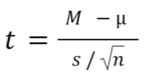
• M: Calculated mean of your sample
• μ: Hypothetical mean you are testing against
• s: The standard deviation of your sample
• n: The number of observations in your sample.

In a one-sample t test, calculating degrees of freedom is simple: one less than the number of objects in your dataset (you’ll see it written as n-1).

Example of a one sample t test

For our example within Prism, we have a dataset of 12 values from an experiment labeled “% of control”. Perhaps these are heights of a sample of plants that have been treated with a new fertilizer. A value of 100 represents the industry-standard control height. Likewise, 123 represents a plant with a height 123% that of the control (that is, 23% larger).

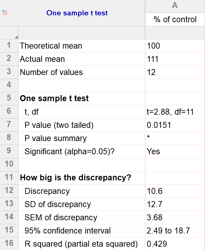
We’ll perform a two-tailed, one-sample t test to see if plants are shorter or taller on average with the fertilizer. We will use a significance threshold of 0.05. Here is the output:

You can see in the output that the actual sample mean was 111. Is that different enough from the industry standard (100) to conclude that there is a statistical difference?

The quick answer is yes, there’s strong evidence that the height of the plants with the fertilizer is greater than the industry standard (p=0.015). The nice thing about using software is that it handles some of the trickier steps for you. In this case, it calculates your test statistic (t=2.88), determines the appropriate degrees of freedom (11), and outputs a P value.

More informative than the P value is the confidence interval of the difference, which is 2.49 to 18.7. The confidence interval tells us that, based on our data, we are confident that the true difference between our sample and the baseline value of 100 is somewhere between 2.49 and 18.7. As long as the difference is statistically significant, the interval will not contain zero.

You can follow these tips for interpreting your own one-sample test.

Graphing a one-sample t test

For some techniques (like regression), graphing the data is a very helpful part of the analysis. For t tests, making a chart of your data is still useful to spot any strange patterns or outliers, but the small sample size means you may already be familiar with any strange things in your data.

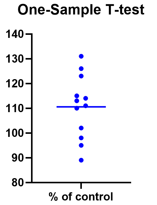
Here we have a simple plot of the data points, perhaps with a mark for the average. We’ve made this as an example, but the truth is that graphing is usually more visually telling for two-sample t tests than for just one sample.

Two sample t tests

There are several kinds of two sample t tests, with the two main categories being paired and unpaired (independent) samples.

Paired samples t test

In a paired samples t test, also called dependent samples t test, there are two samples of data, and each observation in one sample is “paired” with an observation in the second sample. The most common example is when measurements are taken on each subject before and after a treatment. A paired t test example research question is, “Is there a statistical difference between the average red blood cell counts before and after a treatment?”

Having two samples that are closely related simplifies the analysis. Statistical software, such as this paired t test calculator, will simply take a difference between the two values, and then compare that difference to 0.

In some (rare) situations, taking a difference between the pairs violates the assumptions of a t test, because the average difference changes based on the size of the before value (e.g., there’s a larger difference between before and after when there were more to start with). In this case, instead of using a difference test, use a ratio of the before and after values, which is referred to as ratio t tests.

Paired t test formula

The formula for paired samples t test is:

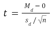
• Md: Mean difference between the samples
• sd: The standard deviation of the differences
• n: The number of differences

Degrees of freedom are the same as before. If you’re studying for an exam, you can remember that the degrees of freedom are still n-1 (not n-2) because we are converting the data into a single column of differences rather than considering the two groups independently.

Also note that the null value here is simply 0. There is no real reason to include “minus 0” in an equation other than to illustrate that we are still doing a hypothesis test. After you take the difference between the two means, you are comparing that difference to 0.

Example

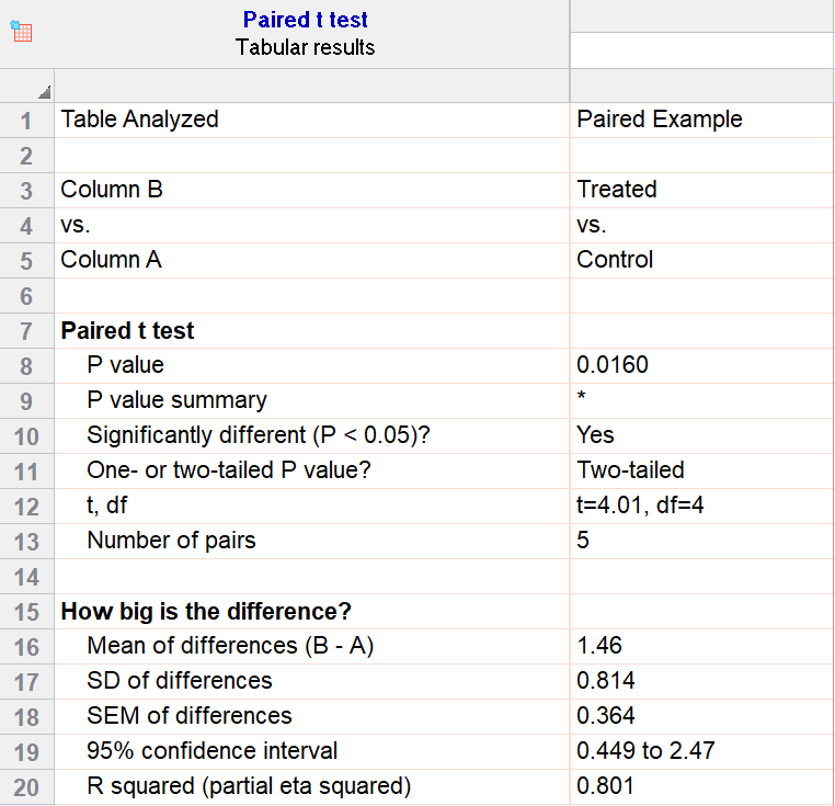
For our example data, we have five test subjects and have taken two measurements from each: before (“control”) and after a treatment (“treated”). If we set alpha = 0.05 and perform a two-tailed test, we observe a statistically significant difference between the treated and control group (p=0.0160, t=4.01, df = 4). We are 95% confident that the true mean difference between the treated and control group is between 0.449 and 2.47.

Graphing a paired t test

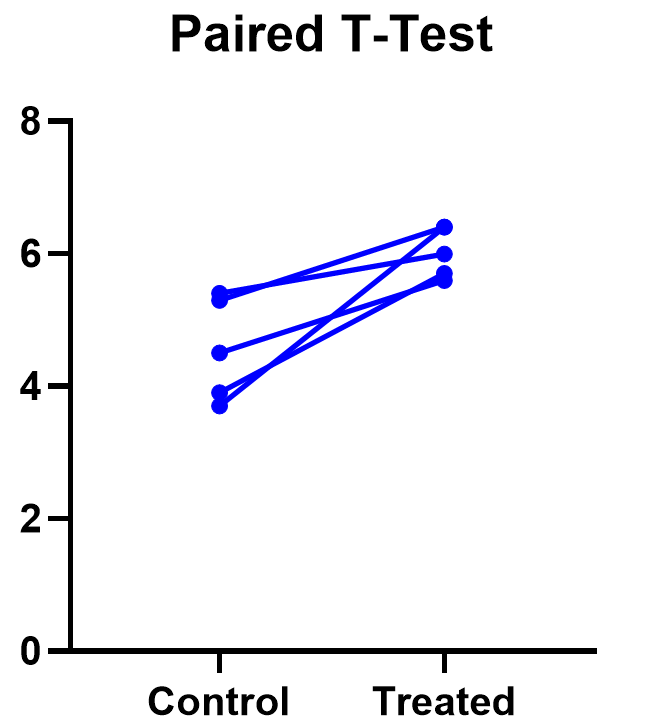
The significant result of the P value suggests evidence that the treatment had some effect, and we can also look at this graphically. The lines that connect the observations can help us spot a pattern, if it exists. In this case the lines show that all observations increased after treatment. While not all graphics are this straightforward, here it is very consistent with the outcome of the t test. 

Prism’s estimation plot is even more helpful because it shows both the data (like above) and the confidence interval for the difference between means. You can easily see the evidence of significance since the confidence interval on the right does not contain zero.

Here are some more graphing tips for paired t tests.

Unpaired samples t test

Unpaired samples t test, also called independent samples t test, is appropriate when you have two sample groups that aren’t correlated with one another. A pharma example is testing a treatment group against a control group of different subjects. Compare that with a paired sample, which might be recording the same subjects before and after a treatment.

With unpaired t tests, in addition to choosing your level of significance and a one or two tailed test, you need to determine whether or not to assume that the variances between the groups are the same or not. If you assume equal variances, then you can “pool” the calculation of the standard error between the two samples. Otherwise, the standard choice is Welch’s t test which corrects for unequal variances. This choice affects the calculation of the test statistic and the power of the test, which is the test’s sensitivity to detect statistical significance. 

It’s best to choose whether or not you’ll use a pooled or unpooled (Welch’s) standard error before running your experiment, because the standard statistical test is notoriously problematic. See more details about unequal variances here.

As long as you’re using statistical software, such as this two-sample t test calculator, it’s just as easy to calculate a test statistic whether or not you assume that the variances of your two samples are the same. If you’re doing it by hand, however, the calculations get more complicated with unequal variances.

Unpaired (independent) samples t test formula

The general two-sample t test formula is:

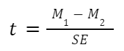
• M1 and M2: Two means you are comparing, one from each dataset
• SE: The combined standard error of the two samples (calculated using pooled or unpooled standard error)

The denominator (standard error) calculation can be complicated, as can the degrees of freedom. If the groups are not balanced (the same number of observations in each), you will need to account for both when determining n for the test as a whole.

Example

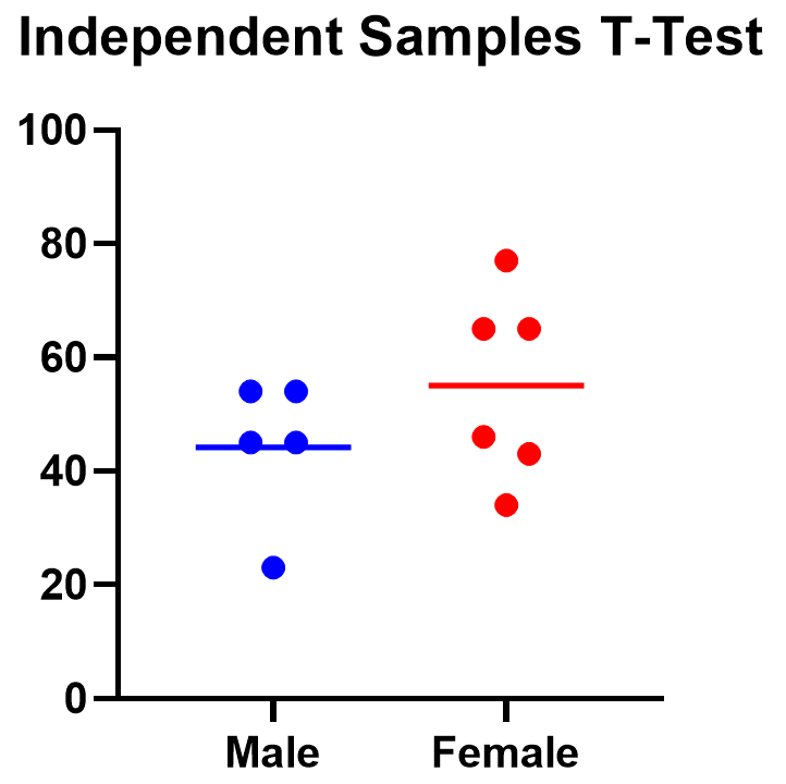
As an example for this family, we conduct a paired samples t test assuming equal variances (pooled). Based on our research hypothesis, we’ll conduct a two-tailed test, and use alpha=0.05 for our level of significance. Our samples were unbalanced, with two samples of 6 and 5 observations respectively. 

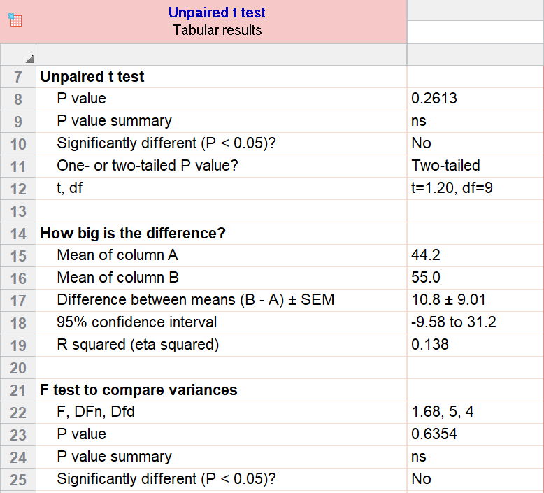
The P value (p=0.261, t = 1.20, df = 9) is higher than our threshold of 0.05. We have not found sufficient evidence to suggest a significant difference. You can see the confidence interval of the difference of the means is -9.58 to 31.2.

Note that the F-test result shows that the variances of the two groups are not significantly different from each other.

Graphing an unpaired samples t test

For an unpaired samples t test, graphing the data can quickly help you get a handle on the two groups and how similar or different they are. Like the paired example, this helps confirm the evidence (or lack thereof) that is found by doing the t test itself.

Below you can see that the observed mean for females is higher than that for males. But because of the variability in the data, we can’t tell if the means are actually different or if the difference is just by chance. 

Nonparametric alternatives for t tests

If your data comes from a normal distribution (or something close enough to a normal distribution), then a t test is valid. If that assumption is violated, you can use nonparametric alternatives.

T tests evaluate whether the mean is different from another value, whereas nonparametric alternatives compare either the median or the rank. Medians are well-known to be much more robust to outliers than the mean.

The downside to nonparametric tests is that they don’t have as much statistical power, meaning a larger difference is required in order to determine that it’s statistically significant.

Wilcoxon signed-rank test

The Wilcoxon signed-rank test is the nonparametric cousin to the one-sample t test. This compares a sample median to a hypothetical median value. It is sometimes erroneously even called the Wilcoxon t test (even though it calculates a “W” statistic).

And if you have two related samples, you should use the Wilcoxon matched pairs test instead. The two versions of Wilcoxon are different, and the matched pairs version is specifically for comparing the median difference for paired samples. 

Mann-Whitney and Kolmogorov-Smirnov tests

For unpaired (independent) samples, there are multiple options for nonparametric testing. Mann-Whitney is more popular and compares the mean ranks (the ordering of values from smallest to largest) of the two samples. Mann-Whitney is often misrepresented as a comparison of medians, but that’s not always the case. Kolmogorov-Smirnov tests if the overall distributions differ between the two samples. 

More t test FAQs

What is the formula for a t test?

The exact formula depends on which type of t test you are running, although there is a basic structure that all t tests have in common. All t test statistics will have the form:

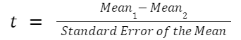
• t: The t test statistic you calculate for your test
• Mean1 and Mean2: Two means you are comparing, at least 1 from your own dataset
• Standard Error of the Mean: The standard error of the mean, also called the standard deviation of the mean, which takes into account the variance and size of your dataset

The exact formula for any t test can be slightly different, particularly the calculation of the standard error. Not only does it matter whether one or two samples are being compared, the relationship between the samples can make a difference too.

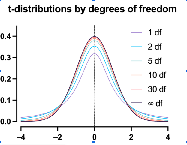
What is a t-distribution?

A t-distribution is similar to a normal distribution. It’s a bell-shaped curve, but compared to a normal it has fatter tails, which means that it’s more common to observe extremes. T-distributions are identified by the number of degrees of freedom. The higher the number, the closer the t-distribution gets to a normal distribution. After about 30 degrees of freedom, a t and a standard normal are practically the same.

t-distribution by degree of freedom

What are degrees of freedom?

Degrees of freedom are a measure of how large your dataset is. They aren’t exactly the number of observations, because they also take into account the number of parameters (e.g., mean, variance) that you have estimated.

What is the difference between paired vs unpaired t tests?

Both paired and unpaired t tests involve two sample groups of data. With a paired t test, the values in each group are related (usually they are before and after values measured on the same test subject). In contrast, with unpaired t tests, the observed values aren’t related between groups. An unpaired, or independent t test, example is comparing the average height of children at school A vs school B. 

When do I use a z-test versus a t test?

Z-tests, which compare data using a normal distribution rather than a t-distribution, are primarily used for two situations. The first is when you’re evaluating proportions (number of failures on an assembly line). The second is when your sample size is large enough (usually around 30) that you can use a normal approximation to evaluate the means.

When should I use ANOVA instead of a t test?

Use ANOVA if you have more than two group means to compare.

What are the differences between t test vs chi square?

Chi square tests are used to evaluate contingency tables, which record a count of the number of subjects that fall into particular categories (e.g., truck, SUV, car). t tests compare the mean(s) of a variable of interest (e.g., height, weight).

What are P values?

P values are the probability that you would get data as or more extreme than the observed data given that the null hypothesis is true. It’s a mouthful, and there are a lot of issues to be aware of with P values.

What are t test critical values?

Critical values are a classical form (they aren’t used directly with modern computing) of determining if a statistical test is significant or not. Historically you could calculate your test statistic from your data, and then use a t-table to look up the cutoff value (critical value) that represented a “significant” result. You would then compare your observed statistic against the critical value.

How do I calculate degrees of freedom for my t test?

In most practical usage, degrees of freedom are the number of observations you have minus the number of parameters you are trying to estimate. The calculation isn’t always straightforward and is approximated for some t tests.

Statistical software calculates degrees of freedom automatically as part of the analysis, so understanding them in more detail isn’t needed beyond assuaging any curiosity.

Perform your own t test

Are you ready to calculate your own t test? Start your 30 day free trial of Prism and get access to:

• A step by step guide on how to perform a t test
• Sample data to save you time
• More tips on how Prism can help your research

With Prism, in a matter of minutes you learn how to go from entering data to performing statistical analyses and generating high-quality graphs.