- Prism
FEATURES
Analyze, graph and present your workComprehensive analysis and statisticsElegant graphing and visualizationsShare, view and discuss your projectsLatest product features and releasesPOPULAR USE CASES
- Enterprise
- Resources
- Support
- Pricing

Ultimate Guide to Survival Analysis
Get all of your Survival Analysis questions answered here.
What is Survival Analysis?
Survival Analysis is a field of statistical tools used to assess the time until an event occurs. As the name implies, this “event” could be death (of humans with a particular disease process, crops or plants under certain conditions, animals, etc.), but it also could be any number of alternatives (the failure of a structural beam or engineering component, the reoccurrence of a disease process, etc.).
For the rest of this article, we’ll look at a fabricated example about the survival rate of domesticated dogs on different diets.
Want to save this for later? Click here to download the eBook
What is survival analysis used for?
Survival analysis is used to describe or predict the survival (or failure) characteristics of a particular population. Often, the researcher is interested in how various treatments or predictor variables affect survival.
Research questions range from general lifespan questions about a population, such as:
- What are the lifespan characteristics of a particular species?
- In a particular setting, such as a country, how long do people live? How does the survival rate change for different age groups such as infants, children, adults, and the elderly?
- In a manufactured product, such as a structural beam, at what load weight do over 1% or 5% of the units fail?
Survival analysis also provides tools to incorporate covariates and other predictors. Some example research questions in this case are:
- How do various factors and covariates (e.g., genetics, diet, exercise, smoking, etc.) affect lifespan?
- Of patients diagnosed with a particular form of cancer, how do various medical treatments affect lifespan, prognosis, or likelihood of remission?
- How do manufacturing processes (e.g., temperature, time, material composition, etc.) affect the failure rate of a product (such as a structural beam)?
See the different uses for Survival Analysis in Prism
What is a survival curve?
A survival curve plots the survival function, which is defined as the probability that the event of interest hasn’t occurred by (and including) each time point.

Survival curve or Kaplan-Meier curve interpretation
With our simulated data, this graph indicates that for Diet 2, after 3 years, 70% of the dogs remain, but after 4 years, only about 25% of dogs on Diet 2 survived. This is strikingly different from Diet 1, which still has 90% surviving after 4 years.
Because the survival curves after 10 years elapsed to have a greater than 0 probability, this plot shows that some values were censored, meaning that some dogs were still alive at the conclusion of the study. With the censored observations, we can’t know for how long they will survive.
In practice, censoring is a very common occurrence. A study is designed and funded for a particular amount of time, with the intention of observing the event of interest, but that might not be the case. Also, dogs, in this case, might come into the study after the study has been running for seven years, so they are only observed for a maximum of three years in this case.
In the discrete case, the survival function at time t, S(t), is S(t) = probability of surviving after (not including) time t
Mathematically, the survival function is 1 - the cumulative distribution function (CDF), or:
S(t) = 1 - F(t) = 1 - Pr {T ≤ t}
This means that in the discrete case, the probability density function (PDF) is the probability of the event occurring at time t.
What is a hazard function?
Hazard functions depict the instantaneous rate of death (or failure) given that an individual has survived up to that time. They are rarely plotted on their own or estimated directly in survival analysis. Instead, they are used behind the scenes in several prominent situations. The most common of these is comparing the ratio of hazards between, say treatment and a control group. Additionally, the hazard function forms the backbone of the calculations and assumptions underlying the very popular Cox proportional hazards model, but even in that situation, the actual hazard functions aren’t of much interest.
Intuitively, hazard functions give you a sense of the risk of the event occurring for an individual at a current point in time. In our demo example, we only recorded data annually, so our data are discrete. This makes the interpretation a little more challenging. Instead of an instantaneous rate of death, we have something close to (but not exactly) an annual rate of death, which we call a “hazard.”

In our example, notice the hazard function for Diet 2 spikes in three locations (ages 4, 8, and 10). This reflects the fact that on the survival curve, more dogs died after 4 years elapsed than remained after 4 years. So clearly, that was a highly hazardous year, and the estimated hazard function value of 1.3 reflects this. Similar situations occurred at years 8 and 10. Even though not nearly as many dogs were surviving at that time, the proportion of dogs that died in years 8 and 10 was relatively large.
In the discrete case, the hazard at time t, h(t), is:

How do I choose a model for survival analysis?
The two most common survival analysis techniques are the Kaplan-Meier method and Cox proportional hazard model.
Both of these require that your data are a sample of independent observations from some “population of interest.” With our example, this means the domesticated dogs are randomly sampled and don’t have confounding effects and relationships with other dogs in the study (such as being from the same litter, breeder, kennel, etc.).
The Kaplan-Meier method is intuitive and nonparametric and therefore requires few assumptions. However, besides a treatment variable (control, treatment 1, treatment 2, …), it cannot easily incorporate additional variables and predictors into the model.
The Cox proportional hazard model, on the other hand, easily incorporates predictor variables, but it is more esoteric. The model has been around for decades, is tried and true, and continues to perform well compared to other alternatives.
What is The Kaplan-Meier method?
The Kaplan-Meier method is the most intuitive model for performing a survival analysis with some added bells and whistles for statistical rigor.
With our example data about domestic dogs on two different diets, we recorded the diet and the year of death of each dog in the study. If we wanted to get an idea of survival rates and probabilities, the most straightforward way to do that would be to just count up how many dogs on each diet died each year. We can also easily aggregate the data to calculate the number of dogs still alive at each time point.
In a nutshell, that’s the basis of the Kaplan-Meier method. It’s called a nonparametric method because there are no distributional assumptions about the data. It’s just a fancy way of tabulating and discussing the results.
If this sounds too simple, you are correct. This perspective oversimplifies Kaplan-Meier, but not by a lot. For example, if some observations in the study don’t experience the event of interest before the study ends, those values need to be represented appropriately in the calculations.
Additionally, statisticians have worked out a mathematical theory that justifies the Kaplan-Meier estimate as being a reasonable choice. Although not all that important in practice (besides giving statisticians like us a job), this provides credence for the method. For example, the Kaplan-Meier estimator for the survival curve is asymptotically unbiased, meaning that as the sample size goes to infinity, the estimator converges on the true value.
When is the Kaplan-Meier method appropriate?
The Kaplan-Meier method is appropriate when you have a fairly simple survival analysis that doesn’t have covariates or other predictor variables. A common example is studying treatment versus control groups. In our simulated data set for this article, we record the survival rate of dogs on two different diets, which is also appropriate here.
However, we have additional (simulated) data about the breed of dogs and their level of activity. Those are likely interesting and important confounding factors in the survival of dogs. We don’t have a way of including them in the analysis with Kaplan-Meier, but we can with the Cox proportional hazards model below.
How do I perform a Kaplan-Meier analysis?
Analyzing Kaplan-Meier can be very simple. All that is needed is the information over time of how long the observational unit or subject was in the study, which group (e.g., treatment, control, etc.) it was in, and whether or not the event occurred or was censored (the event didn’t occur before the end of the study).
See how Prism makes it easy to perform a Kaplan-Meier analysis.
The Kaplan-Meier Curve is an estimate for the survival curve, which is a graphical representation of the proportion of observations that have not experienced the event of interest at each time point.

What is the Cox proportional hazards model?
The industry standard for survival analysis is the Cox proportional hazards model (also called the Cox regression model). To this day, when a new survival model is proposed, researchers compare their model to this one.
It is a robust model, meaning that it works well even if some of the model assumptions are violated. That’s a good thing because the assumptions are difficult to validate empirically, let alone understand.
Rather than modeling the survival curve, which is the approach taken by the Kaplan-Meier method, the Cox model estimates the hazard function. In general, hazard functions are more stable and thus easier to model than survival curves. They depict the hazard, i.e. the instantaneous rate of death (or failure) given that an individual has survived up to that time.
What is the Cox regression model?
It’s just a more ambiguous name for the Cox proportional hazards model.
What are the Cox regression model assumptions?
The prominent assumption with Cox proportional hazards model is that, not surprisingly, the hazard functions are proportional. David Cox noticed that by enforcing that “simple” constraint on the form of the hazard model, a lot of difficult math and unstable optimization can be avoided.
This constraint (that the hazards functions are proportional) also provides an easy way to add in additional variables (covariates) to the model. With our simulated example of dogs on different diets, we can now include the additional information of breed (Great Pyrenees, Labrador, Neapolitan Mastiff) and activity level (Low, Medium, High).
What is the Cox regression model used for?
Because of a clever constraint and the ease at which predictor variables can be added to the model, the Cox proportional hazards model can ascertain hazards and make predictions on data with multiple predictor (covariate) variables. For example, with our simulated data, we could determine the estimated hazard or survival rate of a specific age, breed, and activity level, such as a Great Pyrenees that’s been in the study for three years with a medium activity level.
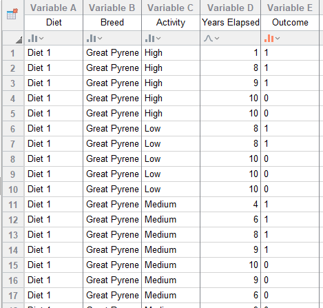
How do I fit a Cox proportional hazard model?
To fit a Cox proportional hazard model, you need to specify the data including time elapsed, outcome (whether that observational unit died or was censored), and any other variables (covariates). In our simulated example data, we are looking at the survival rate of dogs on two different diets, and we include Breed and Activity as additional variables.
Learn how Prism makes it easy to perform Cox Regression.
How do you write a Cox proportional hazard model?
Mathematically, the primary Cox model assumption is that the hazard function, h(t), can be written:

Where i=1pxi*i is a linear combination (a sum) of p predictor (covariate) variables times a regression coefficient. The coefficients and baseline hazard function, h0(t), are estimated using the data.
Another way of saying that the hazard functions are proportional is that the predictor variables’ effects on the hazard function are multiplicative. That’s a major assumption that is difficult to assess.
Unless we include interaction terms (such as activity by breed), this assumes, in our example, that activity level has the same effect on the hazard regardless of how long the dog has been in the study, what breed the dog is, or what diet it is on.
Interaction terms can be included, but greatly complicate interpretation, and introduce multicollinearity, which makes the estimates unstable. As with many statistical models, George Box’s quip that, “All models are wrong but some are useful,” applies here.
The baseline hazard function, h0(t), is key to David Cox’s formulation of the hazard function because that value gets canceled out when taking a ratio of two different hazards (say for Diet 1 vs Diet 2 in our example).

How do you interpret Cox proportional hazards?
Although there are nuances, there are two main options for reporting the results of the Cox proportional hazards model: numerically or graphically.
Numerical results
The most informative part of the numerical results are in the parameter estimates (and hazard ratios). If you are familiar with linear and logistic regression, the interpretation of the numerical results only requires a slight adjustment. The following estimates provide the guts of the information that is needed to understand how each predictor variable affects the hazard functions.
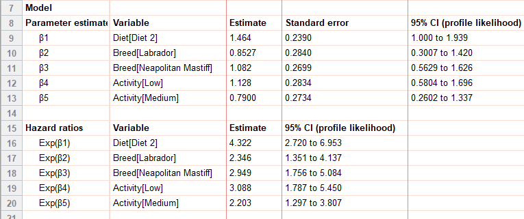
Mathematically, these parameter estimates are used to calculate the hazard function at different values (or levels) of the covariates using the equation:

The Cox model uses the data to find the maximum likelihood estimators for the regression (β) coefficients in the hazard function. Each variable in the model (in our example, these are Diet, Breed, and Activity) has its own regression coefficient and estimate. Categorical variables in the model use reference level coding.
It’s necessary to have a baseline reference with Cox regression models because all of the interpretation is based on calculating proportional hazard functions to the baseline, h0(t).
For our example, the primary question of interest is: Do the two different diets have a significant effect on the survival of dogs? From the parameter estimates and hazard ratio, we can see they do, and, in fact, have quite a drastic difference. In particular (regardless of breed or activity level) dogs on Diet 2 had a 4.322 times higher hazard than dogs on Diet 1, with a 95% confidence interval of (2.720 to 6.953). Because the 95% CI does not include 1, we can also say that this coefficient is statistically significant (p<0.05).
The value we reported above is the hazard ratio, which is just e[ˆβ1] in this case.
What is a hazard ratio?
The hazard ratio is used for interpreting the results of a Cox proportional hazards model and is the multiplicative effect of a variable on the baseline hazard function. For continuous predictor variables, this is the multiplicative effect of a 1-unit change in the predictor (e.g., if weight was a predictor and was measured in kilograms, it would be the multiplicative effect per kilogram). For categorical variables, it is the multiplicative effect that results from that level of the predictor (e.g., Diet 2).
Graphical results
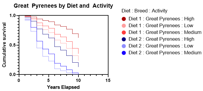
The main graphs for interpretation of the Cox regression model are the cumulative survival functions for specific values of the predictor variables.
There are a number of interesting graphics to look at with our simulated data. For example, the two plots below show the drastic differences between the survival rates of Diet 1 and Diet 2. Here we fixed the activity level at medium and show the differences between breeds by color. Notice the much steeper decline of Diet 2, which indicates a much lower survival rate. Because there aren’t any interaction terms in the model, these survival curves don’t cross. Our data was simulated to behave nicely, and interaction terms weren’t needed. Note that these survival rates per breed are completely fictitious!

A second graphical example looks at the effect of diet and activity level within a single breed (Great Pyrenees). Again, this clearly shows that Diet 1 has a much higher survival rate. It also shows that as the activity level increases, the survival rate increases. Diet 2 is so much worse than Diet 1, that even at a low activity level on Diet 1 there is a higher survival rate than a high activity level on Diet 2.
See how to graph your Survival Analysis results in Prism.
Advantages of Cox proportional hazards model vs logistic regression
The Cox proportional hazards model and a logistic regression model are used for different purposes; they aren’t actually comparable. The Cox proportional hazards model is a tool for survival analysis and measures the time until an event occurs. It is used to compare survival (or failure) rates across different experimental or observational variables. In our example, we look at simulated data on the survival of domesticated dogs on two different diets. We also record information on breed and activity level.
Logistic regression, on the other hand, is a tool for predicting a binary response such as success/failure, present/absent, yes/no. Logistic regression also uses predictor variables, but it’s to ascertain whether or not the event occurs for a specific observational unit. In its standard form, there is no element of time involved in the predictions. You could, for example, use logistic regression to predict whether a student passes a class based on some predictor variables (previous exam scores, age, head circumference, etc.).
Perform Your Own Survival Analysis
Now it’s time to execute your own Survival Analysis according to your specific needs. Start your 30 day free trial of Prism and get access to:
- A step-by-step guide on how to perform Survival Analysis
- Sample data to save you time
- More tips on how Prism can help your research
More than a million scientists in 110 countries rely on Prism to help share their research with the world. With Prism, in a matter of minutes, you learn how to go from entering data to performing statistical analyses and generating high-quality graphs. Start your 30 day trial today or learn more about Survival Analysis in Prism.
Analyze, graph and present your scientific work easily with GraphPad Prism. No coding required.